• Home
• Contact
• Selected works
• Newsfeed
• About
• Search

Bayesian methods are where we need to go. I have pretty strong opinions on this as Bayes provides a way to attune for our prior understanding of the world, move away from null hypothesis testing and take advantage of prior work. Additionally, hierarchical modeling provides a way to collectively pool strength when you have a smaller number of data points. All in all it is a great way to do analysis.

When working with time series analysis, the benefits of Bayesian methods are also great. Bayes provides a way to use an hierarchical modeling approach, and assign probabilities to the outcomes. This super direct way of using uncertainity makes it a nice foil to 95% confidence intervals.

I have take the examples from StichFix’s blog where they contrast the methods of ARIMA and Bayesian Structural Times Series Modeling.

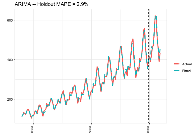
Arima

Autoregressive integrated moving average modeling technique with differencing = 1, and moving average term of 1.

library(lubridate)
library(bsts)
library(dplyr)
library(ggplot2)
library(forecast)


### Load the data
data("AirPassengers")
Y <- window(AirPassengers, start=c(1949, 1), end=c(1959,12))

### Fit the ARIMA model
arima <- arima(log10(Y),
               order=c(0, 1, 1),
               seasonal=list(order=c(0,1,1), period=12))

### Actual versus predicted
d1 <- data.frame(c(10^as.numeric(fitted(arima)), # fitted and predicted
                   10^as.numeric(predict(arima, n.ahead = 12)$pred)),
                   as.numeric(AirPassengers), #actual values
                   as.Date(time(AirPassengers)))
names(d1) <- c("Fitted", "Actual", "Date")


### MAPE (mean absolute percentage error)
MAPE <- filter(d1, year(Date)>1959) %>% summarise(MAPE=mean(abs(Actual-Fitted)/Actual))

### Plot actual versus predicted
ggplot(data=d1, aes(x=Date)) +
  geom_line(aes(y=Actual, colour = "Actual"), size=1.2) +
  geom_line(aes(y=Fitted, colour = "Fitted"), size=1.2, linetype=2) +
  theme_bw() + theme(legend.title = element_blank()) +
  ylab("") + xlab("") +
  geom_vline(xintercept=as.numeric(as.Date("1959-12-01")), linetype=2) +
  ggtitle(paste0("ARIMA -- Holdout MAPE = ", round(100*MAPE,2), "%")) +
  theme(axis.text.x=element_text(angle = -90, hjust = 0))

Bayesian Structural Model

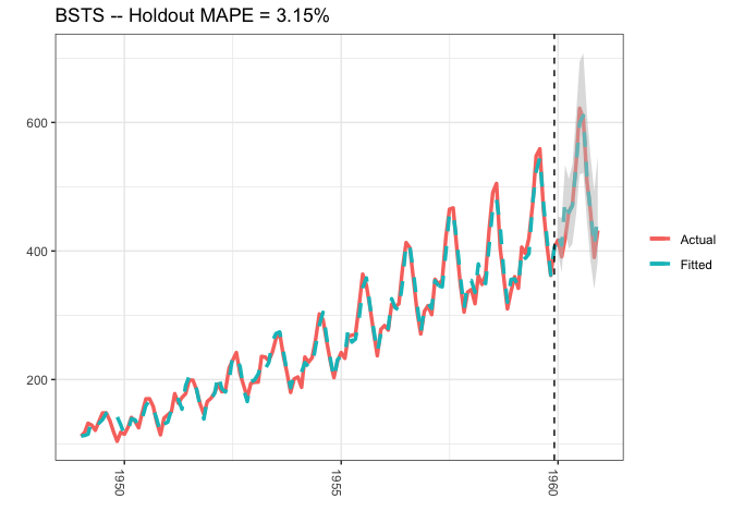
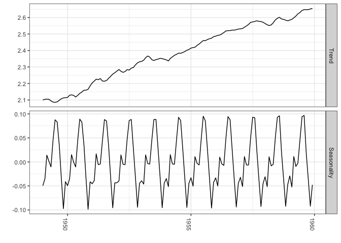
A different approach would be to use a Bayesian structural time series model with unobserved components. This technique is more transparent than ARIMA models and deals with uncertainty in a more elegant manner. It is more transparent because its representation does not rely on differencing, lags and moving averages. You can visually inspect the underlying components of the model. It handles uncertainty in a better way because you can quantify the posterior uncertainty of the individual components, control the variance of the components, and impose prior beliefs on the model. Last, but not least, any ARIMA model can be recast as a structural model.

The model form thus takes:

$$Y_t = \mu + x_t\beta+S_t + e_t$$

$$e_t \sim N(0,\sigma^2_e)$$

$$\mu_{t+1} = \mu_t + v_t$$

$$v_t \sim N(0, \sigma^2_v$$

Here xt denotes a set of regressors, St represents seasonality, and μt is the local level term. The local level term defines how the latent state evolves over time and is often referred to as the unobserved trend. This could, for example, represent an underlying growth in the brand value of a company or external factors that are hard to pinpoint, but it can also soak up short term fluctuations that should be controlled for with explicit terms. Note that the regressor coefficients, seasonality and trend are estimated simultaneously, which helps avoid strange coefficient estimates due to spurious relationships (similar in spirit to Granger causality, see 1). In addition, due to the Bayesian nature of the model, we can shrink the elements of β to promote sparsity or specify outside priors for the means in case we’re not able to get meaningful estimates from the historical data (more on this later).

library(lubridate)
library(bsts)
library(dplyr)
library(ggplot2)

### Load the data
data("AirPassengers")
Y <- window(AirPassengers, start=c(1949, 1), end=c(1959,12))
y <- log10(Y)


### Run the bsts model
ss <- AddLocalLinearTrend(list(), y)
ss <- AddSeasonal(ss, y, nseasons = 12)
bsts.model <- bsts(y, state.specification = ss, niter = 500, ping=0, seed=2016)

### Get a suggested number of burn-ins
burn <- SuggestBurn(0.1, bsts.model)

### Predict
p <- predict.bsts(bsts.model, horizon = 12, burn = burn, quantiles = c(.025, .975))

### Actual versus predicted
d2 <- data.frame(
    # fitted values and predictions
    c(10^as.numeric(-colMeans(bsts.model$one.step.prediction.errors[-(1:burn),])+y),
    10^as.numeric(p$mean)),
    # actual data and dates
    as.numeric(AirPassengers),
    as.Date(time(AirPassengers)))
names(d2) <- c("Fitted", "Actual", "Date")

### MAPE (mean absolute percentage error)
MAPE <- filter(d2, year(Date)>1959) %>% summarise(MAPE=mean(abs(Actual-Fitted)/Actual))

### 95% forecast credible interval
posterior.interval <- cbind.data.frame(
  10^as.numeric(p$interval[1,]),
  10^as.numeric(p$interval[2,]),
  subset(d2, year(Date)>1959)$Date)
names(posterior.interval) <- c("LL", "UL", "Date")

### Join intervals to the forecast
d3 <- left_join(d2, posterior.interval, by="Date")

### Plot actual versus predicted with credible intervals for the holdout period
ggplot(data=d3, aes(x=Date)) +
  geom_line(aes(y=Actual, colour = "Actual"), size=1.2) +
  geom_line(aes(y=Fitted, colour = "Fitted"), size=1.2, linetype=2) +
  theme_bw() + theme(legend.title = element_blank()) + ylab("") + xlab("") +
  geom_vline(xintercept=as.numeric(as.Date("1959-12-01")), linetype=2) +
  geom_ribbon(aes(ymin=LL, ymax=UL), fill="grey", alpha=0.5) +
  ggtitle(paste0("BSTS -- Holdout MAPE = ", round(100*MAPE,2), "%")) +
  theme(axis.text.x=element_text(angle = -90, hjust = 0))

credible.interval <- cbind.data.frame(
  10^as.numeric(apply(p$distribution, 2,function(f){quantile(f,0.75)})),
  10^as.numeric(apply(p$distribution, 2,function(f){median(f)})),
  10^as.numeric(apply(p$distribution, 2,function(f){quantile(f,0.25)})),
  subset(d3, year(Date)>1959)$Date)
names(credible.interval) <- c("p75", "Median", "p25", "Date")

credible.interval %>% knitr::kable(digits = 0)

You can also extract the different components

library(lubridate)
library(bsts)
library(ggplot2)
library(reshape2)

### Set up the model
data("AirPassengers")
Y <- window(AirPassengers, start=c(1949, 1), end=c(1959,12))
y <- log10(Y)
ss <- AddLocalLinearTrend(list(), y)
ss <- AddSeasonal(ss, y, nseasons = 12)
bsts.model <- bsts(y, state.specification = ss, niter = 500, ping=0, seed=2016)

### Get a suggested number of burn-ins
burn <- SuggestBurn(0.1, bsts.model)

### Extract the components
components <- cbind.data.frame(
  colMeans(bsts.model$state.contributions[-(1:burn),"trend",]),
  colMeans(bsts.model$state.contributions[-(1:burn),"seasonal.12.1",]),
  as.Date(time(Y)))
names(components) <- c("Trend", "Seasonality", "Date")
components <- melt(components, id="Date")
names(components) <- c("Date", "Component", "Value")

### Plot
ggplot(data=components, aes(x=Date, y=Value)) + geom_line() +
  theme_bw() + theme(legend.title = element_blank()) + ylab("") + xlab("") +
  facet_grid(Component ~ ., scales="free") + guides(colour=FALSE) +
  theme(axis.text.x=element_text(angle = -90, hjust = 0))

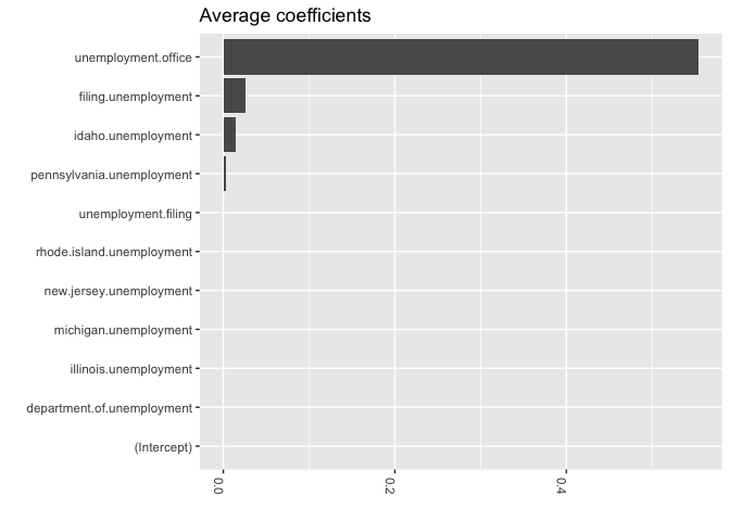
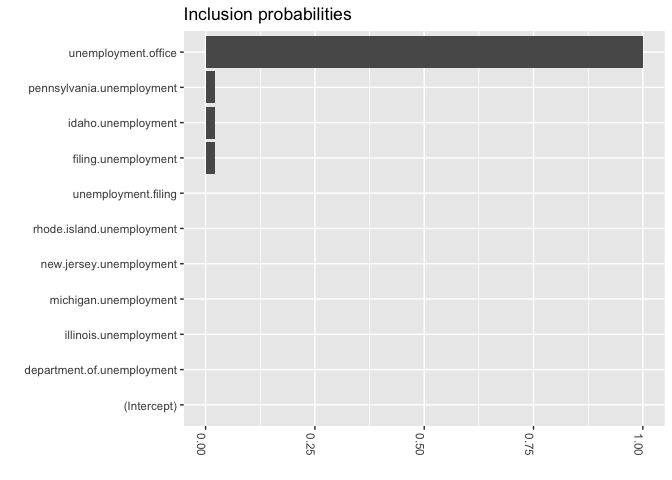
And of course use Bayes for variable selection using the spike and slab method (I was trained to call it stochastic variable selection…but whatever)

library(lubridate)
library(bsts)
library(ggplot2)
library(reshape2)

### Fit the model with regressors
data(iclaims)
ss <- AddLocalLinearTrend(list(), initial.claims$iclaimsNSA)
ss <- AddSeasonal(ss, initial.claims$iclaimsNSA, nseasons = 52)
bsts.reg <- bsts(iclaimsNSA ~ ., state.specification = ss, data =
                initial.claims, niter = 500, ping=0, seed=2016)

### Get the number of burn-ins to discard
burn <- SuggestBurn(0.1, bsts.reg)

### Helper function to get the positive mean of a vector
PositiveMean <- function(b) {
  b <- b[abs(b) > 0]
  if (length(b) > 0)
    return(mean(b))
  return(0)
}

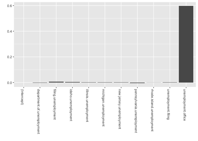
### Get the average coefficients when variables were selected (non-zero slopes)
coeff <- data.frame(melt(apply(bsts.reg$coefficients[-(1:burn),], 2, PositiveMean)))
coeff$Variable <- as.character(row.names(coeff))
ggplot(data=coeff, aes(x=reorder(Variable,value), y=value)) +
  coord_flip()+
  geom_bar(stat="identity", position="identity") +
  theme(axis.text.x=element_text(angle = -90, hjust = 0)) +
  xlab("") + ylab("") + ggtitle("Average coefficients")

### Inclusion probabilities -- i.e., how often were the variables selected
inclusionprobs <- melt(colMeans(bsts.reg$coefficients[-(1:burn),] != 0))
inclusionprobs$Variable <- as.character(row.names(inclusionprobs))
ggplot(data=inclusionprobs, aes(x=reorder(Variable, value), y=value)) +
  geom_bar(stat="identity", position="identity") +
  theme(axis.text.x=element_text(angle = -90, hjust = 0)) +
  coord_flip()+
  xlab("") + ylab("") + ggtitle("Inclusion probabilities")

library(lubridate)
library(bsts)
library(ggplot2)
library(reshape2)

### Fit the model with regressors
data(iclaims)
ss <- AddLocalLinearTrend(list(), initial.claims$iclaimsNSA)
ss <- AddSeasonal(ss, initial.claims$iclaimsNSA, nseasons = 52)
bsts.reg <- bsts(iclaimsNSA ~ ., state.specification = ss, data =
                initial.claims, niter = 500, ping=0, seed=2016)

### Get the number of burn-ins to discard
burn <- SuggestBurn(0.1, bsts.reg)

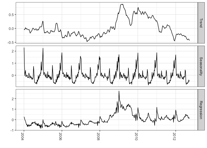
### Get the components
components.withreg <- cbind.data.frame(
  colMeans(bsts.reg$state.contributions[-(1:burn),"trend",]),
  colMeans(bsts.reg$state.contributions[-(1:burn),"seasonal.52.1",]),
  colMeans(bsts.reg$state.contributions[-(1:burn),"regression",]),
  as.Date(time(initial.claims)))
names(components.withreg) <- c("Trend", "Seasonality", "Regression", "Date")
components.withreg <- melt(components.withreg, id.vars="Date")
names(components.withreg) <- c("Date", "Component", "Value")

ggplot(data=components.withreg, aes(x=Date, y=Value)) + geom_line() +
  theme_bw() + theme(legend.title = element_blank()) + ylab("") + xlab("") +
  facet_grid(Component ~ ., scales="free") + guides(colour=FALSE) +
  theme(axis.text.x=element_text(angle = -90, hjust = 0))

And of course adding priors

library(lubridate)
library(bsts)
library(ggplot2)
library(reshape2)

data(iclaims)

prior.spikes <- c(0.1,0.1,0.1,0.1,0.1,0.1,0.1,0.1,0.1,1,0.1)
prior.mean <- c(0,0,0,0,0,0,0,0,0,0.6,0)

### Helper function to get the positive mean of a vector
PositiveMean <- function(b) {
  b <- b[abs(b) > 0]
  if (length(b) > 0)
    return(mean(b))
  return(0)
}

### Set up the priors
prior <- SpikeSlabPrior(x=model.matrix(iclaimsNSA ~ ., data=initial.claims),
                        y=initial.claims$iclaimsNSA,
                        prior.information.weight = 200,
                        prior.inclusion.probabilities = prior.spikes,
                        optional.coefficient.estimate = prior.mean)

### Run the bsts model with the specified priors
data(iclaims)
ss <- AddLocalLinearTrend(list(), initial.claims$iclaimsNSA)
ss <- AddSeasonal(ss, initial.claims$iclaimsNSA, nseasons = 52)
bsts.reg.priors <- bsts(iclaimsNSA ~ ., state.specification = ss,
                        data = initial.claims,
                        niter = 500,
                        prior=prior,
                        ping=0, seed=2016)


### Get the average coefficients when variables were selected (non-zero slopes)
coeff <- data.frame(melt(apply(bsts.reg.priors$coefficients[-(1:burn),], 2, PositiveMean)))
coeff$Variable <- as.character(row.names(coeff))
ggplot(data=coeff, aes(x=Variable, y=value)) +
  geom_bar(stat="identity", position="identity") +
  theme(axis.text.x=element_text(angle = -90, hjust = 0)) +
  xlab("") + ylab("")

So with all of this said we can build Bayesian structural time series models easily, adding prior information, use variable selection and accurately indicate our uncertainity about future predictions. This is pretty powerful stuff. It is also why these techniques are used for anomaly detection and causal inference.

Citation

BibTex citation:

@online{dewitt2018
author = {Michael E. DeWitt},
title = {Bayesian Time Series Analysis with bsts},
date = 2018-07-05,
url = {https://michaeldewittjr.com/articles/2018-07-05-bayesian-time-series-analysis-with-bsts},
langid = {en}
}

For attribution, please cite this work as:

Michael E. DeWitt. 2018. "Bayesian Time Series Analysis with bsts." July 5, 2018. https://michaeldewittjr.com/articles/2018-07-05-bayesian-time-series-analysis-with-bsts