models of microeconomics
Posted onI just wanted to explore a little more some of the topics covered in the fantastic Applied Econometrics with R. All of these examples come from their text in Chapter 3.
Binary Depedent Modeling
  participation   income age education youngkids oldkids foreign
1            no 10.78750 3.0         8         1       1      no
2           yes 10.52425 4.5         8         0       1      no
3            no 10.96858 4.6         9         0       0      no
4            no 11.10500 3.1        11         2       0      no
5            no 11.10847 4.4        12         0       2      no
6           yes 11.02825 4.2        12         0       1      no
swiss_probit <-
Call:
glm(formula = participation ~ . + I(age^2), family = binomial(link = "probit"),
    data = SwissLabor)

Deviance Residuals:
    Min       1Q   Median       3Q      Max
-1.9191  -0.9695  -0.4792   1.0209   2.4803

Coefficients:
            Estimate Std. Error z value Pr(>|z|)
(Intercept)  3.74909    1.40695   2.665  0.00771 **
income      -0.66694    0.13196  -5.054 4.33e-07 ***
age          2.07530    0.40544   5.119 3.08e-07 ***
education    0.01920    0.01793   1.071  0.28428
youngkids   -0.71449    0.10039  -7.117 1.10e-12 ***
oldkids     -0.14698    0.05089  -2.888  0.00387 **
foreignyes   0.71437    0.12133   5.888 3.92e-09 ***
I(age^2)    -0.29434    0.04995  -5.893 3.79e-09 ***
---
Signif. codes:  0 '***' 0.001 '**' 0.01 '*' 0.05 '.' 0.1 ' ' 1

(Dispersion parameter for binomial family taken to be 1)

    Null deviance: 1203.2  on 871  degrees of freedom
Residual deviance: 1017.2  on 864  degrees of freedom
AIC: 1033.2

Number of Fisher Scoring iterations: 4
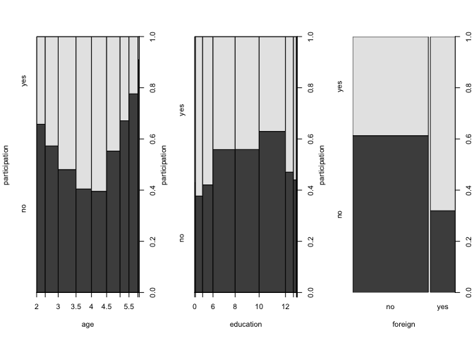
Visualisation of the Data

Retrieving Average Marginal Effects
Average of the sample marginal effects is determined by the following:
fav <-
fav *
 (Intercept)       income          age    education    youngkids      oldkids
 1.241929965 -0.220931858  0.687466185  0.006358743 -0.236682273 -0.048690170
  foreignyes     I(age^2)
 0.236644422 -0.097504844
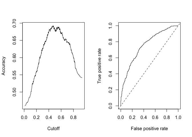
Goodness of Fit
This can be evauluated with a pseudo R2 called _McFadden’s pseudo-R2.
swiss_probit0 <-
1-
[1] 0.1546416
     pred
true    0   1
  no  337 134
  yes 146 255
pred <-

Residuals and Diagnostics
z test of coefficients:

             Estimate Std. Error z value  Pr(>|z|)
(Intercept)  3.749091   1.327072  2.8251  0.004727 **
income      -0.666941   0.127292 -5.2395 1.611e-07 ***
age          2.075297   0.398580  5.2067 1.922e-07 ***
education    0.019196   0.017935  1.0703  0.284479
youngkids   -0.714487   0.106095 -6.7344 1.646e-11 ***
oldkids     -0.146984   0.051609 -2.8480  0.004399 **
foreignyes   0.714373   0.122437  5.8346 5.391e-09 ***
I(age^2)    -0.294344   0.049527 -5.9430 2.798e-09 ***
---
Signif. codes:  0 '***' 0.001 '**' 0.01 '*' 0.05 '.' 0.1 ' ' 1
Count Data
  trips quality ski income userfee  costC   costS   costH
1     0       0 yes      4      no  67.59  68.620  76.800
2     0       0  no      9      no  68.86  70.936  84.780
3     0       0 yes      5      no  58.12  59.465  72.110
4     0       0  no      2      no  15.79  13.750  23.680
5     0       0 yes      3      no  24.02  34.033  34.547
6     0       0 yes      5      no 129.46 137.377 137.850
rd_poisson <-
z test of coefficients:

              Estimate Std. Error  z value  Pr(>|z|)
(Intercept)  0.2649934  0.0937222   2.8274  0.004692 **
quality      0.4717259  0.0170905  27.6016 < 2.2e-16 ***
skiyes       0.4182137  0.0571902   7.3127 2.619e-13 ***
income      -0.1113232  0.0195884  -5.6831 1.323e-08 ***
userfeeyes   0.8981653  0.0789851  11.3713 < 2.2e-16 ***
costC       -0.0034297  0.0031178  -1.1001  0.271309
costS       -0.0425364  0.0016703 -25.4667 < 2.2e-16 ***
costH        0.0361336  0.0027096  13.3353 < 2.2e-16 ***
---
Signif. codes:  0 '***' 0.001 '**' 0.01 '*' 0.05 '.' 0.1 ' ' 1
Overdispersion??
    Overdispersion test

data:  rd_poisson
z = 2.4116, p-value = 0.007941
alternative hypothesis: true dispersion is greater than 1
sample estimates:
dispersion
    6.5658
Yup
    Overdispersion test

data:  rd_poisson
z = 2.9381, p-value = 0.001651
alternative hypothesis: true alpha is greater than 0
sample estimates:
   alpha
1.316051
Negative Binomial
rd_nb <-
z test of coefficients:

              Estimate Std. Error  z value  Pr(>|z|)
(Intercept) -1.1219363  0.2143029  -5.2353 1.647e-07 ***
quality      0.7219990  0.0401165  17.9976 < 2.2e-16 ***
skiyes       0.6121388  0.1503029   4.0727 4.647e-05 ***
income      -0.0260588  0.0424527  -0.6138   0.53933
userfeeyes   0.6691676  0.3530211   1.8955   0.05802 .
costC        0.0480087  0.0091848   5.2270 1.723e-07 ***
costS       -0.0926910  0.0066534 -13.9314 < 2.2e-16 ***
costH        0.0388357  0.0077505   5.0107 5.423e-07 ***
---
Signif. codes:  0 '***' 0.001 '**' 0.01 '*' 0.05 '.' 0.1 ' ' 1
(rd_results <- )
                        [,1]
poisson           -1529.4313
negative_binomial  -825.5576
Improvement!
      0   1  2  3  4  5  6  7  8 9
obs 417  68 38 34 17 13 11  2  8 1
exp 277 146 68 41 30 23 17 13 10 7
This model is under-predicting the zero number of trips. Perhaps it is time to use a zero-inflated model that will help to correct this undercounting.
Thus the linear predictor portion uses all of the independent variables and the inflation component to be a function of quality and income.
rd_zinb <-
Call:
zeroinfl(formula = trips ~ . | quality + income, data = RecreationDemand,
    dist = "negbin")

Pearson residuals:
     Min       1Q   Median       3Q      Max
-1.08868 -0.20032 -0.05687 -0.04525 39.95749

Count model coefficients (negbin with log link):
             Estimate Std. Error z value Pr(>|z|)
(Intercept)  1.096094   0.257075   4.264 2.01e-05 ***
quality      0.169019   0.053135   3.181 0.001468 **
skiyes       0.500479   0.134496   3.721 0.000198 ***
income      -0.069203   0.043802  -1.580 0.114130
userfeeyes   0.542557   0.282819   1.918 0.055062 .
costC        0.040427   0.014522   2.784 0.005372 **
costS       -0.066202   0.007746  -8.547  < 2e-16 ***
costH        0.020609   0.010235   2.014 0.044061 *
Log(theta)   0.189859   0.113134   1.678 0.093312 .

Zero-inflation model coefficients (binomial with logit link):
            Estimate Std. Error z value Pr(>|z|)
(Intercept)   5.7184     1.5596   3.667 0.000246 ***
quality      -8.3596     3.9380  -2.123 0.033768 *
income       -0.2516     0.2847  -0.884 0.376832
---
Signif. codes:  0 '***' 0.001 '**' 0.01 '*' 0.05 '.' 0.1 ' ' 1

Theta = 1.2091
Number of iterations in BFGS optimization: 26
Log-likelihood:  -722 on 12 Df
Let’s check the fit!
      0  1  2  3  4  5  6  7 8 9
obs 417 68 38 34 17 13 11  2 8 1
exp 433 47 35 27 20 16 12 10 8 7
Looks a great deal better!
Hurdle Models
Useful for an excessive number of zeros (or a small number of zeros). This is more widely used in economics according to the text. The hurdle consists of two parts
- Binary part given by a count distribution that is right censored at y = 1 (e.g. is the hurdle crossed)
- A count part given by a left-truncated distribution at y = 1 (e,g, if y > 0, how large is y)
rd_hurdle <-
      0  1  2  3  4  5  6 7 8 9
obs 417 68 38 34 17 13 11 2 8 1
exp 417 74 42 27 19 14 10 8 6 5
Censored Depdent Variables
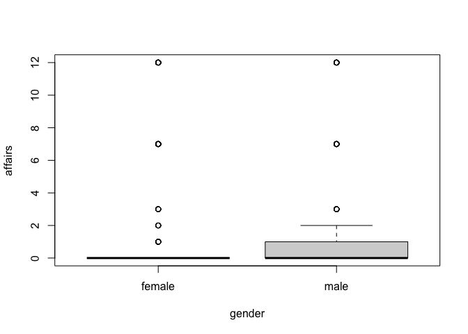
A Tobit model posits that Gaussian linear predictor exists for a latent variable, exists. IT is reported only if the latent variable is positive.
Thus:
   affairs gender age yearsmarried children religiousness education occupation
4        0   male  37        10.00       no             3        18          7
5        0 female  27         4.00       no             4        14          6
11       0 female  32        15.00      yes             1        12          1
16       0   male  57        15.00      yes             5        18          6
23       0   male  22         0.75       no             2        17          6
29       0 female  32         1.50       no             2        17          5
   rating
4       4
5       4
11      4
16      5
23      3
29      5

aff_tob <-
Call:
tobit(formula = affairs ~ age + yearsmarried + religiousness +
    occupation + rating, data = Affairs)

Observations:
         Total  Left-censored     Uncensored Right-censored
           601            451            150              0

Coefficients:
              Estimate Std. Error z value Pr(>|z|)
(Intercept)    8.17420    2.74145   2.982  0.00287 **
age           -0.17933    0.07909  -2.267  0.02337 *
yearsmarried   0.55414    0.13452   4.119 3.80e-05 ***
religiousness -1.68622    0.40375  -4.176 2.96e-05 ***
occupation     0.32605    0.25442   1.282  0.20001
rating        -2.28497    0.40783  -5.603 2.11e-08 ***
Log(scale)     2.10986    0.06710  31.444  < 2e-16 ***
---
Signif. codes:  0 '***' 0.001 '**' 0.01 '*' 0.05 '.' 0.1 ' ' 1

Scale: 8.247

Gaussian distribution
Number of Newton-Raphson Iterations: 4
Log-likelihood: -705.6 on 7 Df
Wald-statistic: 67.71 on 5 Df, p-value: 3.0718e-13
Linear hypothesis test

Hypothesis:
age = 0
occupation = 0

Model 1: restricted model
Model 2: affairs ~ age + yearsmarried + religiousness + occupation + rating

Note: Coefficient covariance matrix supplied.

  Res.Df Df  Chisq Pr(>Chisq)
1    596
2    594  2 4.9078    0.08596 .
---
Signif. codes:  0 '***' 0.001 '**' 0.01 '*' 0.05 '.' 0.1 ' ' 1
Age and occupation are joinly weakyl significant.
Ordinal Response Variables
bank_polr <-
z test of coefficients:

                 Estimate Std. Error z value  Pr(>|z|)
education        0.869998   0.093071  9.3476 < 2.2e-16 ***
minorityyes     -1.056438   0.411994 -2.5642   0.01034 *
custodial|admin  7.951359   1.076932  7.3833 1.544e-13 ***
admin|manage    14.172125   1.474364  9.6124 < 2.2e-16 ***
---
Signif. codes:  0 '***' 0.001 '**' 0.01 '*' 0.05 '.' 0.1 ' ' 1
Citation
BibTex citation:
@online{dewitt2018
author = {Michael E. DeWitt},
title = {models of microeconomics},
date = 2018-09-16,
url = {https://michaeldewittjr.com/articles/2018-09-16-models-of-microeconomics},
langid = {en}
}
For attribution, please cite this work as:
Michael E. DeWitt. 2018. "models of microeconomics." September 16, 2018. https://michaeldewittjr.com/articles/2018-09-16-models-of-microeconomics