MRP using brms
Posted onMulti-Level Regression with Post-Stratification
This blogpost is a reproduction of this. Multi-level regression with post-stratification (MRP) is one of the more powerful predictive strategies for opinion polling and election forecasting. It combines the power of multi-level modeling which anticipate and predict group and population level effects which have good small N predictive properties with post-stratification which helps to temper the predictions to the demographics or other variables of interest. This method has been put out by Andrew Gelman et al and there is a good deal of literature on the subject.
This blog post then seeks to reproduce an example made by Tim Mastny
using the brms package and tidyverse tooling.
Reproduction
#remotes::install_github("hrbrmstr/albersusa")
#library(albersusa)
Data
All the data required to reproduce this example is located here
marriage.data <- foreign::
Statelevel <- foreign::
Census <- foreign::
Tidy and Munge
In this section the data are being cleaned
# add state level predictors to marriage.data
Statelevel <- Statelevel %>%
marriage.data <- Statelevel %>%
%>%
# Combine demographic groups
marriage.data <- marriage.data %>%
%>%
%>%
%>%
Buildign the Post-stratifications
In this step Tim is
# change column names for natural join with marriage.data
Census <- Census %>%
Census <- Statelevel %>%
%>%
Census <- Census %>%
%>%
%>%
Now the fully Bayesian model can be built with the associated group level effects specified.
bayes.mod <-
Examine the model output. If this were for a paper or a real prediction it would be important to run the model through a few more iterations with further diagnostic plots to ensure convergence.
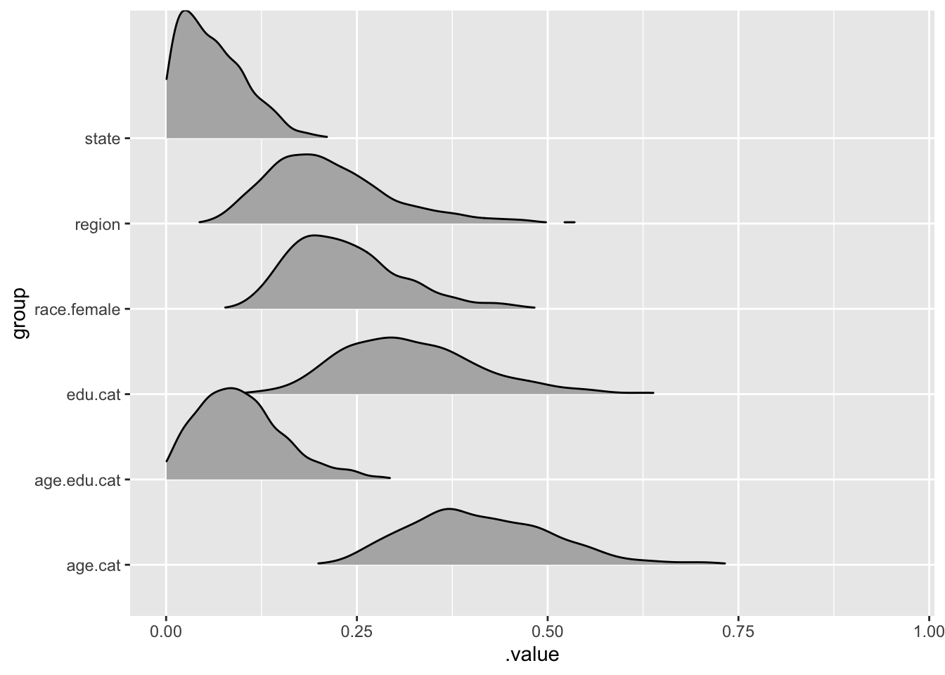
Do some visualisations
bayes.mod %>%
%>%
%>%
%>%
+
ggridges::

Now Bring them Together
The next step then is to combine the predictions from the Bayesian HLM with the postratified values. This can then be used to estimate support.
ps.bayes.mod <- bayes.mod %>%
%>%
%>%
%>%
%>%
%>%
ps.bayes.mod %>%
knitr::
With uncertainity
Now we can add some additional quantification of uncertainity by adding multiple draws from the posterior distribution.
pred<-bayes.mod %>%
%>%
%>%
%>%
%>%
Citation
BibTex citation:
@online{dewitt2018
author = {Michael E. DeWitt},
title = {MRP using brms},
date = 2018-11-07,
url = {https://michaeldewittjr.com/articles/2018-11-07-mrp-using-brms},
langid = {en}
}
For attribution, please cite this work as:
Michael E. DeWitt. 2018. "MRP using brms." November 7, 2018. https://michaeldewittjr.com/articles/2018-11-07-mrp-using-brms