MRP Redux

Posted on April 5^th, 2019

Background

I recently got a question about using MRP and I thought it would be worthwhile to share some of the additional explanation of using this approach with a simulated data set. Simulating your data and testing your method is a really good way to understand if your model is sensitive enough to detect differences. This kind of fake data simulation will allow you to see if your model fails, before using it production or in the field where the cost of failure is high.

Population Data

I’m going to generate some synthetic data for this example. This will represent our population and provide a benchmark for “truth.” The data are completely made up and don’t represent anything in particular.

These data represent a population of 1 million persons, of binary gender, four different races, living in the US. Again, the proportions are made up.

library(tidyverse)
set.seed(336)
n <- 1e6

gender <- sample(c("Female", "Male"), n, replace = TRUE, prob = c(.5,.5))

race <- sample(c("Asian", "Black", "Hispanic", "White"),
               n, replace = TRUE, prob = c(.1, .2, .3, .4))

state <- sample(state.abb, n, replace = T)

Let’s imagine that each person has a probability , $\theta$ of supporting a given opinion. Again, let’s suppose that the probability of support is partially determined by some combination of gender, race, location, and of course some random noise.

base_prob <- ifelse(gender=="Female", .7, .3)
base_prob <- ifelse(race=="Asian", base_prob-.1, base_prob)
base_prob <- ifelse(state %in% c("SC", "NC", "GA", "TX", "FL"),
                    base_prob-.1, base_prob)
base_prob <- base_prob + rnorm(n, 0, .01)
true_opinion <- rbinom(n, 1, base_prob)

population_data <-tibble(
    gender = gender,
    race = race,
    state = state,
    true_opinion = true_opinion
  ) %>%
  left_join(tibble(state.abb, division = state.division), by = c("state" = "state.abb"))

Now I’m going to draw my sample for my analysis. This would represent a completely random sample of my population.

survey <- sample_n(population_data, 500)

Multi-Level Regression

Now we can step into the first component of MRP, the multi-level or hierarchical regression modeling. Here based on literature and inference that race, gender, state, and census division may be important, or help me make inference on the probability of supporting the given option. Additionally, I will use partial pooling to help make inferences for some of the small cell sizes that exist in my survey. I can build that given equation using brms.

library(brms)

my_equation <- bf(true_opinion ~ (1 | race * gender) + (1 | state) + (1 | division))

Now to see what priors I have to set. This step is important as building the above model with lots of variables may have difficulty converging.

get_prior(my_equation, data = survey)

                prior     class      coef       group resp dpar nlpar lb ub
 student_t(3, 0, 2.5) Intercept
 student_t(3, 0, 2.5)        sd                                        0
 student_t(3, 0, 2.5)        sd              division                  0
 student_t(3, 0, 2.5)        sd Intercept    division                  0
 student_t(3, 0, 2.5)        sd                gender                  0
 student_t(3, 0, 2.5)        sd Intercept      gender                  0
 student_t(3, 0, 2.5)        sd                  race                  0
 student_t(3, 0, 2.5)        sd Intercept        race                  0
 student_t(3, 0, 2.5)        sd           race:gender                  0
 student_t(3, 0, 2.5)        sd Intercept race:gender                  0
 student_t(3, 0, 2.5)        sd                 state                  0
 student_t(3, 0, 2.5)        sd Intercept       state                  0
 student_t(3, 0, 2.5)     sigma                                        0
       source
      default
      default
 (vectorized)
 (vectorized)
 (vectorized)
 (vectorized)
 (vectorized)
 (vectorized)
 (vectorized)
 (vectorized)
 (vectorized)
 (vectorized)
      default

Now I can set my priors for the different coefficients in my model.

my_priors <- c(
      set_prior("normal(0,0.2)", class = "sd", group = "race:gender"),
      set_prior("normal(0,0.2)", class = "sd", group = "race"),
      set_prior("normal(0,0.2)", class = "sd", group = "gender"),
      set_prior("normal(0,0.2)", class = "sd", group = "state"),
      set_prior("normal(0,0.2)", class = "sd", group = "division")
    )

Now we can run the model in brms.

fit <- brm(my_equation, survey, prior = my_priors,
           chains = 2, iter = 1000, cores = 2, family = bernoulli(),
           silent = TRUE, backend = "cmdstan")

Running MCMC with 2 parallel chains...

Chain 1 Iteration:   1 / 1000 [  0%]  (Warmup)
Chain 2 Iteration:   1 / 1000 [  0%]  (Warmup)
Chain 1 Iteration: 100 / 1000 [ 10%]  (Warmup)
Chain 2 Iteration: 100 / 1000 [ 10%]  (Warmup)
Chain 1 Iteration: 200 / 1000 [ 20%]  (Warmup)
Chain 2 Iteration: 200 / 1000 [ 20%]  (Warmup)
Chain 2 Iteration: 300 / 1000 [ 30%]  (Warmup)
Chain 1 Iteration: 300 / 1000 [ 30%]  (Warmup)
Chain 2 Iteration: 400 / 1000 [ 40%]  (Warmup)
Chain 1 Iteration: 400 / 1000 [ 40%]  (Warmup)
Chain 2 Iteration: 500 / 1000 [ 50%]  (Warmup)
Chain 2 Iteration: 501 / 1000 [ 50%]  (Sampling)
Chain 1 Iteration: 500 / 1000 [ 50%]  (Warmup)
Chain 1 Iteration: 501 / 1000 [ 50%]  (Sampling)
Chain 2 Iteration: 600 / 1000 [ 60%]  (Sampling)
Chain 1 Iteration: 600 / 1000 [ 60%]  (Sampling)
Chain 2 Iteration: 700 / 1000 [ 70%]  (Sampling)
Chain 1 Iteration: 700 / 1000 [ 70%]  (Sampling)
Chain 2 Iteration: 800 / 1000 [ 80%]  (Sampling)
Chain 1 Iteration: 800 / 1000 [ 80%]  (Sampling)
Chain 2 Iteration: 900 / 1000 [ 90%]  (Sampling)
Chain 2 Iteration: 1000 / 1000 [100%]  (Sampling)
Chain 2 finished in 2.6 seconds.
Chain 1 Iteration: 900 / 1000 [ 90%]  (Sampling)
Chain 1 Iteration: 1000 / 1000 [100%]  (Sampling)
Chain 1 finished in 2.9 seconds.

Both chains finished successfully.
Mean chain execution time: 2.7 seconds.
Total execution time: 3.1 seconds.

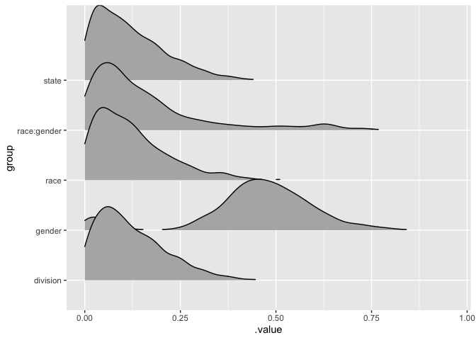
Now we can visualise the outputs.

library(tidybayes)

fit %>%
  gather_draws(`sd_.*`, regex=TRUE) %>%
  ungroup() %>%
  mutate(group = stringr::str_replace_all(.variable, c("sd_" = "","__Intercept"=""))) %>%
  ggplot(aes(y=group, x = .value)) +
  ggridges::geom_density_ridges(aes(height=..density..),
                                rel_min_height = 0.01, stat = "density",
                                scale=1.5)

Additionally, we should do some additional posterior checks which includes checking our Rhat values for convervenges and our effective sample size. Additionally, some posterior predictive checks would also be helpful to ensure that our model is performing well. I won’t do that here, but it is a good practice to do those things.

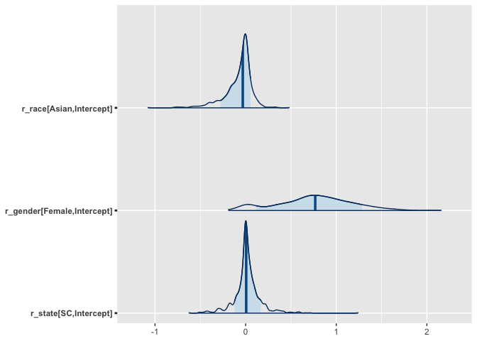
We can also check some of the intercepts to see if the model detected some of the changes that we introduced.

library(bayesplot)
posterior <- as.matrix(fit)

mcmc_areas(posterior,
           pars = c("r_race[Asian,Intercept]",
                    "r_gender[Female,Intercept]",
                    "r_state[SC,Intercept]"),
           prob = 0.8)

It looks like the model picked up the gender differences as well as the specific difference for Asians. However, it looks like the model did not do a great job discriminating on differences for South Carolina. We could explore this further, but it is important to check that our model is performing as expected.

Create the Census Data

Now we step into the post-stratification step. Here we have the population values from our fake data. In reality you would probably use estimates from a census. Here we are interested in predicting state level opinion, so we we want to stratify at that level. If we wanted to make inferences about a different level we would stratify to that given level. I’m going to do both state level overall and race within state for this example.

head(
  post_strat_values <- population_data %>%
    group_by(division, state, race, gender) %>%
    summarise(n = n()) %>%
    group_by(state) %>% # The level at which you want to measure support
    mutate(perc = n / sum(n)) %>%
    ungroup() %>%
    group_by(state, race) %>%
    mutate(perc_2 = n/ sum(n)) %>%
    ungroup(),
    25)

# A tibble: 25 × 7
   division    state race     gender     n   perc perc_2
   <fct>       <chr> <chr>    <chr>  <int>  <dbl>  <dbl>
 1 New England CT    Asian    Female   958 0.0475  0.478
 2 New England CT    Asian    Male    1047 0.0519  0.522
 3 New England CT    Black    Female  2061 0.102   0.509
 4 New England CT    Black    Male    1989 0.0986  0.491
 5 New England CT    Hispanic Female  3053 0.151   0.499
 6 New England CT    Hispanic Male    3060 0.152   0.501
 7 New England CT    White    Female  3997 0.198   0.499
 8 New England CT    White    Male    4009 0.199   0.501
 9 New England MA    Asian    Female   999 0.0493  0.493
10 New England MA    Asian    Male    1026 0.0506  0.507
# ℹ 15 more rows

Now we can add some draws from the posterior distribution to our dataset and then make inferences on them.

pred<-fit %>%
  add_predicted_draws(newdata=post_strat_values, allow_new_levels=TRUE, ndraws = 100) %>%
  mutate(individual_support = .prediction) %>%
   rename(support = .prediction) %>%
  mean_qi() %>%
  mutate(state_support = support * perc) %>% # Post-stratified by state
  mutate(state_race = support *perc_2) # Post-stratified by gender within state

Now we can do whatever we want to do with regard to inferences:

by_state_estimated <- pred %>%
  group_by(state) %>%
  summarise(estimated_support = sum(state_support)) %>%
  left_join(population_data %>%
              group_by(state) %>%
              summarise(true_support = mean(true_opinion)))

by_state_estimated_2 <- pred %>%
  group_by(state) %>%
  summarise(estimated_support = sum(state_support)) %>%
  left_join(population_data %>%
              group_by(state) %>%
              summarise(true_support = mean(true_opinion))) %>%
  left_join(survey %>%
              group_by(state) %>%
              summarise(survey_support = mean(true_opinion))) %>%
  gather(method, prediction, -true_support, - state)

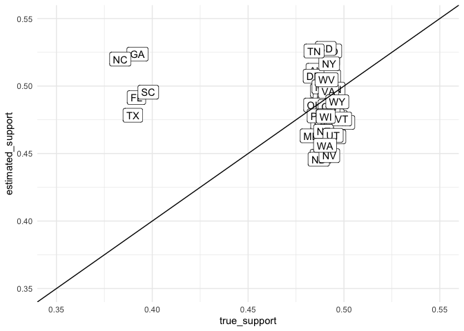
Now we can look to see how our prediction did for the population, though we missed the Southern states. Probably because our decision to partial pool on division was a bad one given the effects we introduced at the state level did not necessarily coincide with the census division.

by_state_estimated %>%
ggplot(aes(true_support, estimated_support, label = state))+
  geom_label()+
  geom_abline(slope = 1)+
  theme_minimal()+
  xlim(.35,.55)+
  ylim(.35,.55)

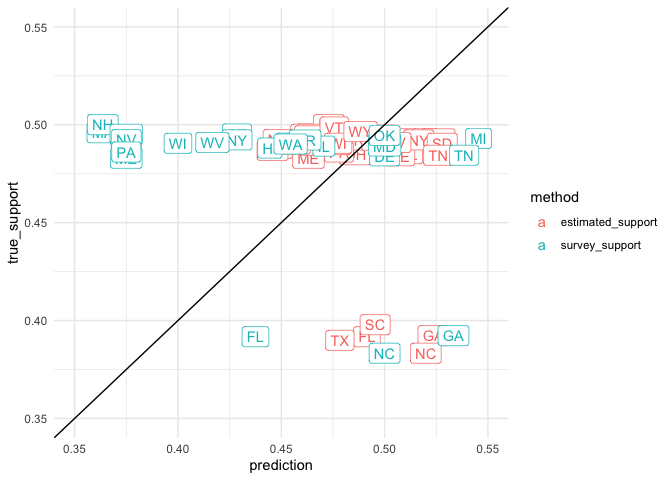
But we can at least be calmed by the fact that if we made direct prediction from our survey we would have been way wrong!

by_state_estimated_2 %>%
  ggplot(aes(prediction, true_support, color = method, label = state))+
  geom_label()+
  geom_abline(slope = 1)+
  theme_minimal()+
  xlim(.35,.55)+
  ylim(.35,.55)

Looking at support by Race within a given community requires that we use a different post-stratification variable which we created earlier.

(by_state_race_estimated <- pred %>%
  group_by(state, race) %>%
  summarise(estimated_support = sum(state_race)) %>%
  left_join(population_data %>%
              group_by(state, race) %>%
              summarise(true_support = mean(true_opinion))))

# A tibble: 200 × 4
# Groups:   state [50]
   state race     estimated_support true_support
   <chr> <chr>                <dbl>        <dbl>
 1 AK    Asian                0.487        0.396
 2 AK    Black                0.499        0.494
 3 AK    Hispanic             0.470        0.496
 4 AK    White                0.481        0.508
 5 AL    Asian                0.458        0.388
 6 AL    Black                0.511        0.500
 7 AL    Hispanic             0.535        0.492
 8 AL    White                0.509        0.498
 9 AR    Asian                0.481        0.395
10 AR    Black                0.473        0.496
# ℹ 190 more rows

Citation

BibTex citation:

@online{dewitt2019
author = {Michael E. DeWitt},
title = {MRP Redux},
date = 2019-04-05,
url = {https://michaeldewittjr.com/articles/2019-04-05-mrp-redux},
langid = {en}
}

For attribution, please cite this work as:

Michael E. DeWitt. 2019. "MRP Redux." April 5, 2019. https://michaeldewittjr.com/articles/2019-04-05-mrp-redux