Prospective Outbreak Detection and Aberration Algorithms
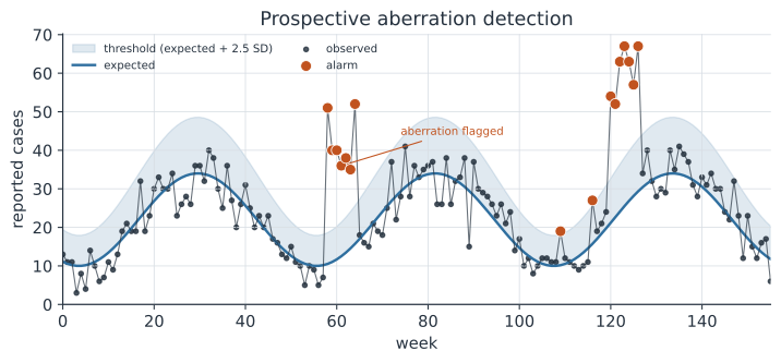
A public health surveillance system watches many disease-and-place time series at once, and no analyst can eyeball them all every week. The task is prospective aberration detection: at each new time point, decide whether the latest count is higher than recent history leads you to expect, and if so, raise an alarm for a human to investigate. This is statistical process control adapted to noisy, seasonal, count-valued public health data, and it is what turns a stream of reports into a timely signal.
Prospective, not retrospective#
Aberration detection differs from the spatial cluster detection done after the fact on a closed dataset. Here the series is open-ended and each week arrives one at a time, so the method must decide now, using only data up to the present, and it is judged on timeliness and false-alarm rate rather than on a single retrospective test. The generic recipe is the same across algorithms: from recent history build an expected count and a measure of its variability, form a threshold, and alarm when the observed count crosses it. The algorithms differ in how they estimate the expectation and how much memory they carry.
A family of algorithms#
Shewhart charts compare the current count to a mean plus a multiple of the standard deviation estimated from a baseline window; they react fast to large single-week spikes but miss slow build-ups.
CUSUM (cumulative sum) charts accumulate the running excess of observed over expected, so a series of small exceedances adds up to an alarm; they are more sensitive to gradual shifts at the cost of slower response to a one-week jump.
The EARS methods (Early Aberration Reporting System) are deliberately simple, using only a short trailing baseline of the preceding few weeks, which makes them robust when little history exists — for a new syndrome or a new reporting stream.
The Farrington algorithm is the most fully specified: it fits an overdispersed Poisson or quasi-Poisson regression to counts from comparable weeks in previous years, including a time trend and reweighting past outbreaks downward, then predicts the current week and sets a threshold from the upper prediction interval (Farrington et al. 1996, doi:10.2307/2983331).
It is the backbone of routine infectious disease monitoring at several national agencies, and these algorithms are collected in the surveillance package for R (Salmon, Schumacher & Höhle 2016, doi:10.18637/jss.v070.i10).
Reading the threshold#
An alarm is a hypothesis, not a conclusion. The threshold trades sensitivity against specificity: a lower threshold catches more real outbreaks but cries wolf more often, and with hundreds of series monitored weekly even a small false-alarm probability produces many alarms to triage. Seasonality and secular trends must be modeled or the algorithm will alarm every winter, and past outbreaks in the baseline must be down-weighted or the system quietly learns to expect them and stops reacting. A raised alarm feeds into outbreak investigation; a well-tuned system is one an overworked epidemiologist can trust enough to act on.
A worked example#
We take a weekly count series and apply a simple EARS-style rule. The baseline is the mean and standard deviation of the seven preceding weeks; the statistic is the standardized excess of the current week, and we alarm when it exceeds three.
In code#
R#
counts <- c(5, 7, 6, 8, 6, 7, 9, 8, 7, 24)   # last value is the current week

baseline <- counts[(length(counts) - 7):(length(counts) - 1)]
mu <- mean(baseline); s <- sd(baseline)
current <- counts[length(counts)]
C1 <- (current - mu) / s          # EARS C1 statistic

c(expected = mu, statistic = C1, alarm = C1 > 3)
Python#
import numpy as np

counts = np.array([5, 7, 6, 8, 6, 7, 9, 8, 7, 24.0])  # last = current week

baseline = counts[-8:-1]
mu, s = baseline.mean(), baseline.std(ddof=1)
current = counts[-1]
c1 = (current - mu) / s            # EARS C1 statistic

print(f"expected  = {mu:.2f}")
print(f"statistic = {c1:.2f}")
print(f"alarm     = {c1 > 3}")
expected  = 7.29
statistic = 15.02
alarm     = True
Julia#
using Statistics

counts = [5, 7, 6, 8, 6, 7, 9, 8, 7, 24.0]   # last = current week

baseline = counts[end-7:end-1]
mu, s = mean(baseline), std(baseline)
current = counts[end]
C1 = (current - mu) / s            # EARS C1 statistic

(expected = mu, statistic = C1, alarm = C1 > 3)
Why it matters#
Prospective aberration detection is how surveillance scales: it lets a handful of epidemiologists monitor thousands of series and spend their attention where the data say something has changed. The choice of algorithm and threshold is a policy decision disguised as a statistical one, because it sets how many outbreaks are caught early against how many false alarms the system generates. Understanding that the expectation must absorb seasonality and past outbreaks, and that the threshold encodes a sensitivity-specificity trade-off, is what separates an alarm worth chasing from noise.
Related#
- Surveillance Systems — the data streams these algorithms watch
- Outbreak Investigation — what happens after an alarm
- Spatial Cluster Detection — the where, after the fact
- Nowcasting and Reporting Delays — correcting recent counts before testing them
- Generalized Linear Models — the Poisson baseline behind Farrington