Age, Period, and Cohort Effects
Risk almost always changes with age, but not all age patterns are about age. Some are about cohort: the group of people born in the same period, who share early-life exposures, immunological history, and behaviors that follow them through life. A risk model that treats age as the whole story can attribute to biology a pattern that is really the fingerprint of a particular generation.
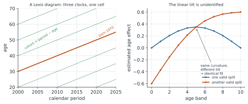
Three timescales, one observation#
Any individual carries three clocks that move together.
- Age — time since birth, the driver of biological and immune maturation.
- Period — the calendar time of observation, capturing everything that acts on everyone at once (a new vaccine, a pandemic year, a change in case definition).
- Cohort — the year (or interval) of birth, capturing exposures that mark a generation for life (childhood infection, diet, smoking norms, the pathogen circulating when their immune system was first trained).
Cohort effects are why influenza mortality by age can show a bump that tracks a birth year rather than an age: the generation first exposed to a particular flu subtype in childhood carries an imprinted susceptibility (or protection) for decades, a phenomenon called antigenic imprinting or original antigenic sin. The same logic applies to smoking-related cancers, where risk by age looks very different for cohorts who took up smoking young than for those who never did.
The identification problem#
The reason cohort effects are hard is not conceptual but arithmetic. The three clocks are exactly linearly dependent:
Knowing any two fixes the third. So if a model includes a linear term for each of age, period, and cohort, their columns are collinear and the individual linear slopes are not identified: you can add a constant to the age trend, subtract it from the cohort trend, and add it to the period trend and get exactly the same fitted values (Figure 1). No amount of data breaks this tie, because it is a property of the design, not of sampling noise.
What is and is not estimable#
The good news is that the collinearity is only in the linear trends. Anything that does not move in lockstep with a straight line survives. Estimable quantities include the overall fit, the curvature (second differences) of each effect, and the deviations of each age, period, or cohort from its own linear trend. What is not estimable, without an outside assumption, is how to divide the single overall linear drift among the three axes. This is the honest framing: the data tell you the shape of each effect but not the tilt, and any method that reports a clean linear age, period, and cohort slope has smuggled in a constraint somewhere.
Strategies for risk models#
Several approaches let you fit an age-period-cohort (APC) model, each buying identification with a different assumption.
- Drop or constrain one axis. If theory says period has no linear trend (say, no secular change in ascertainment), fit age and cohort and let period enter only through curvature. The result is only as trustworthy as that assumption.
- Equality constraints. Force two adjacent groups to share an effect (e.g. the first two cohorts are equal). This identifies the model but the answer moves as you move the constraint, so report the sensitivity.
- Curvature-only reporting. Report the estimable pieces — second differences, local slopes, deviations from linearity — and refuse to report the unidentified linear split. This is the most defensible choice when the science does not pin down a constraint.
- The intrinsic estimator. A principled way to pick the one solution orthogonal to the null vector of the design; it is reproducible but its estimand still depends on the coding, so it is not a free lunch.
- Smooth / partial-pooling models. Treat age, period, and cohort as smooth functions (splines) or as random effects in a cross-classified multilevel model. Smoothness and shrinkage act as soft constraints and are often the most stable choice for prediction, though they still do not manufacture information the design lacks.
When you can ignore cohort#
Cohort matters when exposure is tied to birth year, not to current age or current calendar time. For a pathogen where risk is set by current susceptibility and current contact patterns — most acute respiratory and enteric infections — an age term plus a period term usually captures the structure, and forcing a cohort axis in only adds an unidentified degree of freedom. Reach for a full APC model when you have a mechanism for lifelong imprinting: early-life infection, immune priming, or a durable behavioral cohort like a vaccination-era generation.
A worked example: the collinearity is real#
The clearest demonstration is that the age-period-cohort design matrix is rank-deficient by construction. Lay out a Lexis grid of age groups by calendar periods, form the birth cohort as period minus age, and the three centered linear columns have rank two, not three.
import numpy as np

ages    = np.arange(30, 71, 10)      # 30, 40, 50, 60, 70
periods = np.arange(2000, 2021, 5)   # 2000, 2005, ..., 2020

grid   = np.array([(a, p, p - a) for a in ages for p in periods], float)
grid_c = grid - grid.mean(axis=0)    # center each column

print("columns: age, period, cohort")
print("rank of the three linear terms:", np.linalg.matrix_rank(grid_c))
print("age + cohort - period (all zero):",
      np.round(grid_c[:, 0] + grid_c[:, 2] - grid_c[:, 1], 6)[:5])
columns: age, period, cohort
rank of the three linear terms: 2
age + cohort - period (all zero): [0. 0. 0. 0. 0.]
The rank is two because the third column is a fixed combination of the other two, and the printed vector confirms in every cell. A regression that includes all three linear terms therefore has an infinitude of equally good coefficient triples; only functions that are constant across that ambiguity (curvatures and deviations) are pinned down.
In code#
R#
ages    <- seq(30, 70, by = 10)
periods <- seq(2000, 2020, by = 5)
grid    <- expand.grid(age = ages, period = periods)
grid$cohort <- grid$period - grid$age

# center and check the rank of the three linear terms
X  <- scale(as.matrix(grid[, c("age", "period", "cohort")]), scale = FALSE)
qr(X)$rank                     # 2, not 3 -> linear APC is unidentified

# the Epi / apc packages fit identifiable reparameterizations
# (drift + curvatures) rather than raw linear slopes
Python#
import numpy as np
import statsmodels.api as sm

ages    = np.arange(30, 71, 10)
periods = np.arange(2000, 2021, 5)
grid    = np.array([(a, p, p - a) for a in ages for p in periods], float)

# a full linear APC design (with intercept) is rank-deficient
X = sm.add_constant(grid)
print("design columns:", X.shape[1], "-> rank:", np.linalg.matrix_rank(X))
design columns: 4 -> rank: 3
Julia#
ages    = 30:10:70
periods = 2000:5:2020
grid = [(a, p, p - a) for a in ages for p in periods]
M = reduce(vcat, [ [a p c] for (a, p, c) in grid ])
Mc = M .- sum(M, dims = 1) ./ size(M, 1)   # center
using LinearAlgebra
rank(Mc)                                    # 2, not 3
Why it matters#
Confusing a cohort effect for an age effect leads to bad extrapolation: you project a generation’s imprinted risk onto every future generation as if it were a fact of aging. Getting the decomposition right — or, more honestly, reporting only the pieces the data can support and being explicit about the constraint that identifies the rest — is what separates a defensible risk model from one that has quietly assumed away the hardest part of the problem.