Bayesian Bandits for Adaptive Sampling and Trial Design

Suppose you can afford to run 1,000 tests across four surveillance sites, and you care about finding cases — not about estimating every site equally well. A fixed design splits the budget evenly and never learns; a purely greedy design pours everything into whichever site looked best after the first few tests and can be fooled by noise. A Bayesian bandit threads the needle: it keeps a posterior on each site’s positivity, and each round it allocates the next test in proportion to the probability that a site is the best one — automatically shifting resources toward the hot site while still occasionally probing the others in case it was wrong.

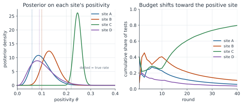
This is the multi-armed bandit problem: each “arm” (site, treatment, ad, dose) pays off with an unknown probability, and every pull is both a chance to earn a reward and a chance to learn. The tension between those two goals is the exploration–exploitation trade-off, and the elegant Bayesian answer to it is Thompson sampling.

The setup: arms, rewards, and beliefs#

We have $K$ arms (here $K=4$ sites). Pulling arm $k$ yields a Bernoulli reward — a positive test — with unknown probability $\theta_k$. Our goal over a horizon of $T$ pulls is to maximize the expected number of positives found, $\sum_{t} \theta_{a_t}$, where $a_t \in \{1,\dots,K\}$ is the arm chosen at step $t$.

Because each arm is a proportion, the natural belief to carry is a Beta distribution, which is conjugate to the Binomial likelihood. Start each site with a prior $\text{Beta}(\alpha_k, \beta_k)$ — a uniform $\text{Beta}(1,1)$ if you know nothing. After observing $s_k$ positives in $n_k$ tests at that site, the posterior is simply

$$\theta_k \mid \text{data} \;\sim\; \text{Beta}\!\left(\alpha_k + s_k,\; \beta_k + n_k - s_k\right). \tag{1}$$

The two hyperparameters have a clean reading: $\alpha_k - 1$ is (prior plus observed) positives, $\beta_k - 1$ is negatives, and the posterior mean is $\hat\theta_k = \alpha_k / (\alpha_k + \beta_k)$. The total count $\alpha_k + \beta_k$ is the effective sample size — how sharp the belief is.

Thompson sampling: probability matching#

Given those posteriors, how should we choose the next site? Thompson sampling (posterior sampling) is almost embarrassingly simple:

1. Draw one sample $\tilde\theta_k \sim \text{Beta}(\alpha_k,\beta_k)$ from each arm’s current posterior.
2. Pull the arm with the largest sample, $a = \arg\max_k \tilde\theta_k$.
3. Observe the reward, update that arm’s posterior via (1), and repeat.

The magic is that the probability an arm gets pulled equals the posterior probability that it is genuinely the best arm. Early on, when posteriors are wide, the draws are noisy and every arm gets tried — that is exploration, and it is automatic, requiring no tuning parameter. As evidence sharpens the posteriors, the best arm wins the draw more and more often — that is exploitation, and it emerges from the same one line of code. This property is called probability matching.

There is rarely a need to evaluate the integral in (2) directly — that is the point. Drawing one sample per arm and taking the argmax is a Monte Carlo estimate of pulling each arm with probability $w_k$, and it costs one random draw per arm.

Measuring how well it does: regret#

The yardstick for a bandit policy is regret — the reward you forfeited by not always pulling the truly-best arm $\theta^\* = \max_k \theta_k$:

$$\text{Regret}(T) \;=\; \sum_{t=1}^{T} \big(\theta^\* - \theta_{a_t}\big) \;=\; \sum_{k} \Delta_k\, N_k(T), \qquad \Delta_k = \theta^\* - \theta_k ,$$

where $N_k(T)$ is the number of times arm $k$ was pulled and $\Delta_k$ is its suboptimality gap. A policy that never learns (uniform allocation) pays regret growing linearly in $T$, because it keeps pulling bad arms at a fixed rate. Thompson sampling achieves logarithmic regret, $\mathbb{E}[\text{Regret}(T)] = O(\log T)$ — matching the Lai–Robbins lower bound on what any policy can achieve — because the number of pulls it wastes on each inferior arm grows only like $\log T$. In the survey setting, low regret means more positives found for the same number of tests.

The updating process, step by step#

The loop that produces Figure 1 is worth spelling out, because every adaptive design in this family is a variation on it.

1. Initialize a posterior $\text{Beta}(\alpha_k,\beta_k)$ for each of the four sites (start uniform, or encode prior surveillance data).
2. Sample a plausible positivity $\tilde\theta_k$ from each posterior.
3. Allocate the next test (or batch of tests) to the site(s) with the highest sampled positivity.
4. Observe how many of those tests come back positive.
5. Update the chosen site’s posterior: add positives to $\alpha_k$, negatives to $\beta_k$.
6. Repeat until the budget is spent.

Because the update in step 5 is just addition, the whole procedure is cheap enough to run on a phone in the field, and it is fully sequential: new data change the allocation on the very next round. The only real design choices are the priors (step 1) and the batch size (step 3) — larger batches update less often but parallelize the field work.

Worked example: four sites#

Take four sites with true (unknown) positivities $\theta = (0.06, 0.10, 0.22, 0.09)$ — site C is the hot spot. Start every site at $\text{Beta}(1,1)$ and run 40 rounds of 25 tests, drawing a Thompson allocation for each test. After the first few rounds the posteriors are still wide and the budget is spread fairly evenly; by round 40 close to 80% of all tests have gone to site C, its posterior is tight around 0.22, and the neglected sites keep wide posteriors — we are confident about the winner and deliberately uncertain about the also-rans, which is exactly the right allocation of certainty when the goal is finding cases. Compare that to an even split, which would have spent 250 tests on each site and found far fewer positives.

In code#

R#

A complete Thompson-sampling loop over the four sites, with per-test re-draws inside each batch.

set.seed(1)
p_true <- c(A = 0.06, B = 0.10, C = 0.22, D = 0.09)  # unknown to the sampler
K <- length(p_true)
a <- rep(1, K); b <- rep(1, K)                        # Beta(1,1) priors

rounds <- 40; batch <- 25
for (t in seq_len(rounds)) {
  # Thompson sampling: each test goes to the site with the largest posterior draw
  draws  <- matrix(rbeta(batch * K, a, b), nrow = batch, byrow = TRUE)
  picks  <- max.col(draws)                            # argmax per test
  for (k in seq_len(K)) {
    n_k <- sum(picks == k)
    if (n_k > 0) {
      y_k <- rbinom(1, n_k, p_true[k])                # positives observed
      a[k] <- a[k] + y_k                              # update: add positives
      b[k] <- b[k] + n_k - y_k                        #         add negatives
    }
  }
}

post_mean <- a / (a + b)
n_tests   <- (a - 1) + (b - 1)
round(rbind(posterior_mean = post_mean, tests_used = n_tests), 3)
# site C draws most of the budget and its posterior mean sits near 0.22

Python#

The same loop, executed at build time so the numbers are real.

import numpy as np

rng = np.random.default_rng(20260711)
p_true = np.array([0.06, 0.10, 0.22, 0.09])   # sites A, B, C, D — unknown
sites = ["A", "B", "C", "D"]
K = len(p_true)
a = np.ones(K)          # Beta(1,1) priors: alpha = 1 + positives
b = np.ones(K)          #                   beta  = 1 + negatives

rounds, batch = 40, 25
for t in range(rounds):
    # one posterior draw per test, then send each test to its argmax site
    draws = rng.beta(a[None, :], b[None, :], size=(batch, K))
    picks = draws.argmax(axis=1)
    for k in range(K):
        n_k = int((picks == k).sum())
        if n_k:
            y_k = rng.binomial(n_k, p_true[k])   # positives found
            a[k] += y_k                          # conjugate update
            b[k] += n_k - y_k

post_mean = a / (a + b)
tests = (a - 1) + (b - 1)
for k in range(K):
    print(f"site {sites[k]}: {int(tests[k]):4d} tests, "
          f"posterior mean {post_mean[k]:.3f}")
print(f"total positives found: {int((a - 1).sum())} / {int(tests.sum())} tests")

site A:   58 tests, posterior mean 0.100
site B:  108 tests, posterior mean 0.136
site C:  797 tests, posterior mean 0.247
site D:   37 tests, posterior mean 0.103
total positives found: 218 / 1000 tests

Julia#

using Random, Distributions
Random.seed!(1)

p_true = [0.06, 0.10, 0.22, 0.09]          # sites A, B, C, D
K = length(p_true)
a = ones(K); b = ones(K)                   # Beta(1,1) priors

rounds, batch = 40, 25
for t in 1:rounds
    picks = [argmax(rand.(Beta.(a, b))) for _ in 1:batch]  # Thompson per test
    for k in 1:K
        n_k = count(==(k), picks)
        if n_k > 0
            y_k = rand(Binomial(n_k, p_true[k]))           # positives
            a[k] += y_k                                    # add positives
            b[k] += n_k - y_k                              # add negatives
        end
    end
end

println("posterior means: ", round.(a ./ (a .+ b), digits = 3))
println("tests per site:  ", Int.((a .- 1) .+ (b .- 1)))

The allocation probability directly#

If you want the exact probability each site is best — the $w_k$ of (2) — a few thousand joint posterior draws estimate it without evaluating the integral. This is also how you report “there is a 94% chance site C has the highest positivity.”

def prob_best(a, b, draws=20000, seed=0):
    rng = np.random.default_rng(seed)
    samples = rng.beta(a, b, size=(draws, len(a)))   # joint posterior draws
    winners = samples.argmax(axis=1)
    return np.bincount(winners, minlength=len(a)) / draws

w = prob_best(a, b)
for k in range(K):
    print(f"P(site {sites[k]} is best) = {w[k]:.3f}")

P(site A is best) = 0.002
P(site B is best) = 0.002
P(site C is best) = 0.986
P(site D is best) = 0.010

A week-by-week playbook: 100 tests over 8 weeks#

The abstract loop above updates after every test; in the field you usually update on a fixed cadence. Here is the concrete operating procedure for a program with 100 tests every week for an 8-week season across the same four sites, and it is exactly what a field team would follow with a spreadsheet.

• Week 1 — even warm start. With no data yet, split the budget evenly: 25 tests to each site. You cannot adapt to evidence you do not have, so week 1 just seeds every posterior.
• Weeks 2–8 — adapt. Before each week, (1) guarantee every site a floor of 5 tests so you never stop watching a site, then (2) hand out the remaining 80 tests by Thompson sampling — draw a posterior sample for each of the 80 and send each test to the site with the highest draw. A site the posteriors currently favor collects most of those 80; a site that has looked quiet collects only its floor of 5.
• End of each week — update. Fold the week’s positives and negatives into each site’s Beta posterior (add positives to $\alpha$, negatives to $\beta$), and repeat.

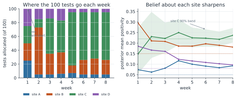
Running this with true positivities $\theta = (0.05, 0.15, 0.22, 0.08)$ for sites A–D — a deliberately harder season where sites B and C are close — produces the allocation below.

import numpy as np

rng = np.random.default_rng(1)
theta = np.array([0.05, 0.15, 0.22, 0.08])   # sites A, B, C, D — unknown
K, weeks, weekly, floor = 4, 8, 100, 5
flex = weekly - floor * K                     # 80 tests steered by Thompson
a, b = np.ones(K), np.ones(K)

print("week   A   B   C   D   positives")
total_pos = 0
for w in range(weeks):
    if w == 0:
        alloc = np.full(K, weekly // K)       # even warm start: 25 each
    else:
        alloc = np.full(K, floor)             # floor: keep watching every site
        picks = rng.beta(a[None, :], b[None, :], size=(flex, K)).argmax(axis=1)
        for k in range(K):
            alloc[k] += int((picks == k).sum())   # Thompson-allocate the 80
    pos = np.array([rng.binomial(int(alloc[k]), theta[k]) for k in range(K)])
    a += pos                                   # conjugate update: + positives
    b += alloc - pos                           #                   + negatives
    total_pos += int(pos.sum())
    row = " ".join(f"{int(alloc[k]):>3d}" for k in range(K))
    print(f"  {w + 1:>2}  {row}   {int(pos.sum()):>4d}")

print(f"adaptive: {total_pos} positives found in {weeks * weekly} tests")
print(f"even 25/site/week would expect ~{int(weeks * weekly / K * theta.sum())}")

week   A   B   C   D   positives
   1   25  25  25  25     15
   2    5  68  12  15     19
   3    5  30  51  14     20
   4    6  31  46  17     19
   5    7  11  77   5     16
   6    5  21  69   5     21
   7    5  23  67   5     16
   8    5  21  69   5     26
adaptive: 152 positives found in 800 tests
even 25/site/week would expect ~100

Read the table top to bottom and you can watch the algorithm think:

• Week 1 is the even 25/25/25/25 split — pure warm start.
• Week 2 pours 68 tests into site B, not C: by luck B returned the most positives in week 1, so its posterior temporarily led. This is the bandit chasing the early front-runner — and it is supposed to, given what it knew.
• Weeks 3–4 are the correction: as site C’s own positives accumulate, its posterior climbs and it takes 51 then 46 tests while B cools to the low 30s. The two contenders are still genuinely competing.
• Week 5 is the turning point — C pulls away to 77 tests and B collapses to 11, because the evidence has finally separated $\theta_C \approx 0.22$ from $\theta_B \approx 0.15$.
• Weeks 6–8 settle: C holds a steady ~65–70 tests a week, B keeps ~20 (it is the second-best site, not a dead one, so it still earns real allocation), and A and D sit at their floor of 5.

The key lesson is that a single noisy week did not lock in the wrong answer: the floor kept C alive when it looked mediocre in week 2, and continued updating steered the budget back to the truth. Over the full season the adaptive design finds 152 positives against the even split’s expected ~100 — roughly a 50% larger yield from the very same 800 tests — because it spent most of its budget on the two genuinely higher-positivity sites instead of burning a quarter of every week on the two quiet ones.

The same weekly loop in R#

set.seed(1)
theta <- c(A = 0.05, B = 0.15, C = 0.22, D = 0.08)   # unknown to the sampler
K <- 4; weeks <- 8; weekly <- 100; floor <- 5
flex <- weekly - floor * K                            # 80 steered by Thompson
a <- rep(1, K); b <- rep(1, K)

alloc_tbl <- matrix(0L, weeks, K, dimnames = list(paste0("wk", 1:weeks), names(theta)))
for (w in seq_len(weeks)) {
  if (w == 1) {
    alloc <- rep(weekly %/% K, K)                     # even warm start: 25 each
  } else {
    alloc <- rep(floor, K)                            # floor for every site
    draws <- matrix(rbeta(flex * K, a, b), nrow = flex, byrow = TRUE)
    picks <- max.col(draws)                           # Thompson for the 80
    for (k in seq_len(K)) alloc[k] <- alloc[k] + sum(picks == k)
  }
  pos <- rbinom(K, alloc, theta)                      # positives per site
  a <- a + pos; b <- b + alloc - pos                  # conjugate update
  alloc_tbl[w, ] <- alloc
}
alloc_tbl        # rows = weeks, columns = tests sent to each site

And in Julia#

using Random, Distributions
Random.seed!(1)

theta = [0.05, 0.15, 0.22, 0.08]                 # sites A, B, C, D
K, weeks, weekly, floor = 4, 8, 100, 5
flex = weekly - floor * K                         # 80 steered by Thompson
a = ones(K); b = ones(K)

for w in 1:weeks
    if w == 1
        alloc = fill(weekly ÷ K, K)               # even warm start: 25 each
    else
        alloc = fill(floor, K)                    # floor for every site
        picks = [argmax(rand.(Beta.(a, b))) for _ in 1:flex]
        for k in 1:K
            alloc[k] += count(==(k), picks)       # Thompson-allocate the 80
        end
    end
    pos = [rand(Binomial(alloc[k], theta[k])) for k in 1:K]
    a .+= pos; b .+= alloc .- pos                 # conjugate update
    println("week $w: ", alloc, "  positives ", sum(pos))
end

From surveillance to the clinic: adaptive trial design#

Swap “sites” for “treatment arms” and “positive test” for “patient responded,” and the identical machinery becomes response-adaptive randomization (RAR) — the engine of Bayesian adaptive clinical trials. Instead of fixing a 1:1:1:1 allocation for the whole study, you update a posterior on each arm’s success probability as outcomes arrive and steer new patients toward the arms that are winning. The ethical appeal is direct: fewer trial participants are assigned to inferior treatments, because the allocation follows the accumulating evidence.

The clinical setting adds a few refinements to the bare bandit:

• Tempered allocation. Pure Thompson sampling can allocate very aggressively; trials often temper it, pulling arm $k$ with probability $\propto \big[\Pr(\text{arm } k \text{ best})\big]^{c}$ for some $0 < c < 1$, or clamping allocation away from 0 so every arm keeps accruing enough data for a valid final comparison.
• Posterior stopping rules. Rather than a fixed sample size, the trial stops for superiority when $\Pr(\theta_A > \theta_B \mid \text{data})$ crosses a high threshold (say 0.99), or for futility when it falls below a low one — a genuinely sequential design that can end early when the answer is clear.
• Arm dropping and adding. Multi-arm, multi-stage (platform) trials drop arms whose posterior probability of being best decays, and can add new arms mid-study, all under the same updating rule.

Response-adaptive randomization has real history: the 1980s ECMO trial for newborns used a “play-the-winner” adaptive rule and assigned all but one infant to the treatment that was working, and modern platform trials — I-SPY 2 in breast cancer, REMAP-CAP in pneumonia and COVID-19 — run many arms under exactly this Bayesian-updating framework, dropping and adding treatments as posteriors evolve. The survey-sampling bandit and the adaptive trial are the same algorithm pointed at different rewards.

Why it matters#

The Bayesian bandit turns a static allocation problem into a learning loop: carry a posterior on each option, act in proportion to the probability each option is best, and let the data reshape the allocation. For surveillance it means finding more cases per test by concentrating limited diagnostic capacity where the signal is, without a human re-deciding the split each week. For clinical research it means trials that expose fewer patients to worse treatments and can stop as soon as the evidence is decisive. The whole apparatus rests on two ideas this site returns to again and again — conjugate updating to make learning cheap, and posterior probabilities as the currency of decisions — which is what lets one short loop serve both the field epidemiologist and the trialist.

Related#

• Bayesian Inference — the priors, likelihood, and posterior the bandit updates
• Binomial Distribution — the Beta–Binomial conjugate pair at the core
• Survey Sampling — fixed designs the bandit adapts away from
• Optimal Experimental Design — allocating effort to learn most efficiently
• Experimental Design — randomization, bias, and study structure
• Markov Chain Monte Carlo — sampling posteriors when conjugacy fails
• Diagnostic Testing and Screening — what a “positive” means
• Quantitative Methods