Competing Risks

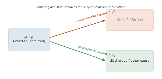
Standard survival analysis tracks one event and treats everything else as censoring. But often several events compete: a hospitalized patient may die of the infection, or be discharged, or die of something else, and the first to happen removes them from risk of the others. Treating a competing event as ordinary censoring — as if the patient could still, counterfactually, have the event of interest later — silently assumes it away, and overestimates how often the event of interest occurs.

Figure 1. A subject starts at risk and moves to exactly one of two absorbing states, each with its own cause-specific hazard. Entering one state removes them from risk of the other, so the events compete and each cause needs its own cumulative incidence function.

Two kinds of hazard#

With competing events there is no single “the” hazard; there are two useful ones, and they answer different questions.

The cause-specific hazard $\lambda_k(t)$ is the instantaneous rate of event $k$ among those still event-free and at risk. It is what a Cox model fit to cause $k$ (censoring the competing events) estimates, and it is the right target for etiology — does a covariate change the rate at which this cause strikes?
The subdistribution hazard (Fine–Gray) keeps subjects who had a competing event in the risk set, so it maps directly onto the cumulative incidence. It is the right target for prediction — does a covariate change the probability a patient ends up with this outcome?

The two can even point in opposite directions, which is not a paradox: a treatment can leave the infection-death rate untouched yet lower its incidence by speeding discharge.

The cumulative incidence function#

The quantity you actually want is the cumulative incidence function (CIF) — the probability of having had cause $k$ by time $t$ , accounting for the competing events. It is built from the cause-specific hazard weighted by overall survival (the Aalen–Johansen estimator):

$\text{CIF}_k(t) = \sum_{s \le t} S(s^-)\,\frac{d_k(s)}{Y(s)},$

where $S$ is all-cause survival, $d_k$ the cause- $k$ events, and $Y$ the number at risk. Because $S$ falls as any cause removes subjects, the CIFs of all causes add up to $1 - S(t)$ and never exceed one.

Warning

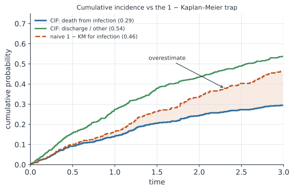
The common shortcut of reporting $1 - \text{KM}$ for one cause (Kaplan–Meier with the competing event censored) overestimates the cumulative incidence, sometimes badly, because it credits the event-of-interest with hazard the competing event never allowed to play out (Figure 2). Use the cumulative incidence function, not $1 - \text{KM}$ .

Figure 2. The cumulative incidence functions for two competing events rise to account for everyone who left the at-risk state; the naive 1 − Kaplan–Meier curve for the infection death (dashed) sits well above the correct cumulative incidence.

A worked example#

Patients are at risk of death from infection (cause 1, rate depending on a high-risk marker $Z$ ) or discharge/other (cause 2), with follow-up truncated at $t=3$ .

Python

import numpy as np
from statsmodels.duration.hazard_regression import PHReg

rng = np.random.default_rng(6)
n = 700
Z = rng.binomial(1, 0.5, n)                       # high-risk marker
T1 = rng.exponential(1 / (0.15 * np.exp(0.7 * Z)), n)   # time to infection death
T2 = rng.exponential(1 / 0.35, n)                        # time to discharge/other
Tstar = np.minimum(T1, T2)
cause = np.where(T1 <= T2, 1, 2)
obs = np.minimum(Tstar, 3.0)                      # administrative censoring at t=3
cause = np.where(Tstar <= 3.0, cause, 0)          # 0 = still at risk (censored)

# cumulative incidence (Aalen-Johansen) vs the naive 1 - KM
S = 1.0; cif1 = 0.0; km1 = 1.0
for t in np.unique(obs[cause > 0]):
    Y = (obs >= t).sum()
    d1 = ((obs == t) & (cause == 1)).sum(); d = ((obs == t) & (cause > 0)).sum()
    cif1 += S * d1 / Y; km1 *= (1 - d1 / Y); S *= (1 - d / Y)
print(f"CIF (infection death)  {cif1:.3f}")
print(f"naive 1 - KM           {1 - km1:.3f}   <- overestimate")

# cause-specific hazard: Cox for cause 1, competing event censored
m = PHReg(obs, Z.reshape(-1, 1), status=(cause == 1).astype(int)).fit()
print(f"cause-specific HR for Z: {np.exp(m.params[0]):.2f}")

CIF (infection death)  0.294
naive 1 - KM           0.464   <- overestimate
cause-specific HR for Z: 2.09

The correct cumulative incidence of infection death is well below the naive $1-\text{KM}$ — the discrepancy is exactly the discharges that the naive method pretends could still become infection deaths. The cause-specific Cox model recovers the elevated hazard in the high-risk group; for a statement about cumulative risk by group, a Fine–Gray subdistribution model would be fit instead.

In code#

R#

library(survival)
# cumulative incidence functions for all causes at once
fit <- survfit(Surv(time, factor(cause)) ~ 1, data = d)   # Aalen-Johansen CIF
# cause-specific Cox (etiology):
coxph(Surv(time, cause == 1) ~ Z, data = d)
library(cmprsk)      # Fine-Gray subdistribution model (prediction):
crr(d$time, d$cause, cov1 = d$Z, failcode = 1)

Julia#

Julia

using Survival
# cause-specific hazards via Cox on each cause (competing events censored);
# the cumulative incidence follows from the Aalen-Johansen estimator

Why it matters#

Competing risks are the rule, not the exception, in infectious-disease outcomes: in-hospital mortality competes with discharge, death from the infection competes with death from comorbidity, progression competes with cure. Reporting $1 - \text{KM}$ for one of these — still distressingly common — overstates the risk and can distort everything downstream, from prognostic counseling to trial sample sizes. Getting it right means naming the competing events, reporting cumulative incidence rather than $1 - \text{KM}$ , and choosing the cause-specific hazard for questions about mechanism and the subdistribution hazard for questions about a patient’s absolute risk.