Critical Transitions and Early-Warning Signals

Many ecological and epidemiological systems can flip abruptly between states when a slowly changing condition crosses a threshold, and the flip often looks sudden even though the approach was gradual. The reason is critical slowing down: as the system nears a fold (saddle-node) bifurcation, its recovery from small perturbations gets sluggish, and that sluggishness leaves generic statistical fingerprints in the fluctuations before anything visibly changes. Rising variance and rising lag-1 autocorrelation are the headline signals, and because they are generic they work for a pathogen drifting toward emergence ($R_0\to1$ from below) just as well as for a lake tipping into a turbid state.

Critical slowing down

Consider a scalar system $\dot{x}=f(x,\mu)$ with a stable equilibrium $x^\star(\mu)$. Near that equilibrium the recovery rate from a small perturbation is set by the linearization, the eigenvalue $\rho=\partial f/\partial x$ evaluated at $x^\star$, and stability requires $\rho<0$. The characteristic return time after a nudge is $1/|\rho|$, so the closer $\rho$ sits to zero, the longer the system takes to relax back.

At a saddle-node bifurcation the equilibrium is about to vanish, and there $f(x^\star)=0$ and $\partial f/\partial x=0$ simultaneously. The normal form $\dot{x}=\mu-x^2$ makes this concrete: the stable branch is $x^\star=\sqrt{\mu}$, the eigenvalue is $\rho=-2\sqrt{\mu}$, and as $\mu\to0$ the recovery rate $\rho\to0$ while the return time $1/|\rho|\to\infty$. The system slows to a crawl exactly as it approaches the tipping point.

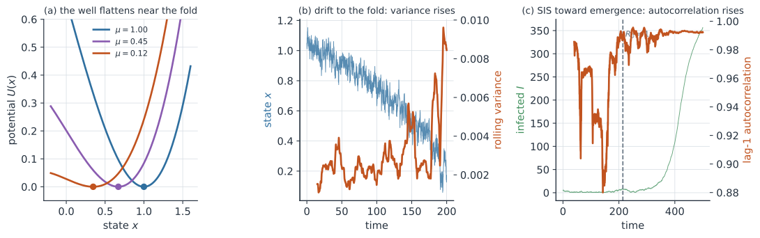
Picture the dynamics as a ball in a potential well, $\dot{x}=-\,\mathrm{d}U/\mathrm{d}x$. Far from the bifurcation the well is steep and the ball returns quickly; as $\mu$ drops the well flattens, and near the fold it becomes almost level so the ball drifts sluggishly and wanders far under any push. This flattening well is the mechanical picture behind every early-warning signal.

The leading indicators

Real systems are perturbed continuously by noise, so write the stochastic version $\mathrm{d}x=f(x,\mu)\,\mathrm{d}t+\sigma\,\mathrm{d}W$ and linearize around $x^\star$ to get an Ornstein–Uhlenbeck process with return rate $|\rho|$. Its stationary variance is $\sigma^2/(2|\rho|)$, which blows up as $|\rho|\to0$: a flatter well lets the same noise push the state further from equilibrium. Sampled at interval $\Delta t$, its lag-1 autocorrelation is $\rho_1=e^{-|\rho|\Delta t}$, which climbs toward $1$ as recovery slows because each observation carries more memory of the last.

So the two robust fingerprints of an approaching fold are rising variance and rising lag-1 autocorrelation ($\rho_1\to1$). When the potential well is asymmetric the state spends more time on its shallow side, which shows up as a growing skewness of the fluctuations. In spatial systems the same slowdown inflates spatial correlation, as neighboring locations relax together rather than independently (Scheffer et al. 2009 doi:10.1038/nature08227).

Alternative stable states and hysteresis

Folds matter because they underlie alternative stable states: over a range of the control parameter the system has two stable equilibria separated by an unstable one, and which state you observe depends on history. Push the parameter past the fold and the current state disappears, so the system drops catastrophically to the remaining alternative — a regime shift (Scheffer et al. 2001 doi:10.1038/35098000). Not every transition is like this; smooth transitions track the parameter continuously and reverse just as smoothly, whereas fold-driven ones jump.

The signature of the catastrophic case is hysteresis: reversing the parameter does not retrace the collapse, because the system now sits in the alternative basin and must be pushed back past a different fold to recover. This is why degraded states are sticky and why early warning is worth having: once the shift happens, undoing it can require driving the condition far beyond where the collapse began.

Epidemiological application

The disease-ecology payoff is that emergence and elimination are both fold-like approaches to $R_0=1$. A slowly forced SIS or SIR model with $R_0$ drifting upward toward $1$ from below sits near its disease-free equilibrium, and as $R_0\to1$ that equilibrium loses stability, so case counts show critical slowing down before sustained transmission takes off (Brett et al. 2017 doi:10.1098/rsif.2017.0115). Drive $R_0$ downward toward $1$ from above and the endemic equilibrium slows in the same way, so the indicators also rise on the road to elimination.

The caveats are real and worth stating. The signals are trends in noisy statistics, so they demand careful detrending, a sensible rolling-window bandwidth, and enough data before the transition to establish a baseline. False positives are common, autocorrelation can rise for reasons unrelated to a fold, and the effective reproduction number estimated directly is often a more actionable target when case data are good; early-warning indicators are best read as a complementary, model-light signal rather than a standalone alarm.

A worked example

Simulate the fold normal form $\mathrm{d}x=(\mu-x^2)\,\mathrm{d}t+\sigma\,\mathrm{d}W$ with $\sigma=0.09$ while $\mu$ ramps slowly from $1.1$ down to $0.03$, tracking the stable branch $x^\star=\sqrt{\mu}$. Compute the variance and lag-1 autocorrelation in a $300$-step rolling window, then summarize each trend with Kendall’s $\tau$ (the rank correlation with time, so $\tau>0$ means a monotone rise). Both statistics come out clearly positive — variance $\tau\approx+0.38$ and autocorrelation $\tau\approx+0.34$ — confirming that the fluctuations swell and grow more autocorrelated as the fold nears, even though the mean state has barely moved.

In code

We integrate the fold SDE with Euler–Maruyama, roll the two indicators, and test their trend with Kendall’s $\tau$.

R

set.seed(1834)
n <- 4000; dt <- 0.05; sigma <- 0.09
mu <- seq(1.1, 0.03, length.out = n)
x <- numeric(n); x[1] <- sqrt(mu[1])
for (k in 2:n) {
  drift <- mu[k - 1] - x[k - 1]^2
  x[k] <- x[k - 1] + drift * dt + sigma * sqrt(dt) * rnorm(1)
}

win <- 300
roll <- function(a, f) sapply(seq(win, length(a)),
                              function(k) f(a[(k - win + 1):k]))
ar1 <- function(s) { s <- s - mean(s); sum(s[-1] * s[-length(s)]) / sum(s^2) }
v <- roll(x, var); r <- roll(x, ar1)
cor(seq_along(v), v, method = "kendall")   # variance trend, tau > 0
cor(seq_along(r), r, method = "kendall")   # autocorrelation trend, tau > 0

Python

import numpy as np
from scipy.stats import kendalltau

rng = np.random.default_rng(1834)

# Scalar SDE dx = (mu - x^2) dt + sigma dW, a saddle-node (fold) normal form.
# mu drifts down toward the fold at mu = 0 (stable branch x = sqrt(mu)).
n, dt, sigma = 4000, 0.05, 0.09
mu = np.linspace(1.1, 0.03, n)
x = np.empty(n); x[0] = np.sqrt(mu[0])
for k in range(1, n):
    drift = mu[k - 1] - x[k - 1] ** 2
    x[k] = x[k - 1] + drift * dt + sigma * np.sqrt(dt) * rng.standard_normal()

def roll(a, win, fn):
    return np.array([fn(a[k - win:k]) for k in range(win, a.size)])

def ar1(seg):
    s = seg - seg.mean()
    return np.sum(s[1:] * s[:-1]) / np.sum(s * s)

var = roll(x, 300, np.var)
rho = roll(x, 300, ar1)
tt = np.arange(var.size)
print(f"variance trend:              Kendall tau = {kendalltau(tt, var).statistic:+.2f}")
print(f"lag-1 autocorrelation trend: Kendall tau = {kendalltau(tt, rho).statistic:+.2f}")
print("both rise as the fold nears (critical slowing down)")

variance trend:              Kendall tau = +0.38
lag-1 autocorrelation trend: Kendall tau = +0.34
both rise as the fold nears (critical slowing down)

Julia

using Random, Statistics, StatsBase

Random.seed!(1834)
n = 4000; dt = 0.05; sigma = 0.09
mu = range(1.1, 0.03; length = n)
x = zeros(n); x[1] = sqrt(mu[1])
for k in 2:n
    drift = mu[k - 1] - x[k - 1]^2
    x[k] = x[k - 1] + drift * dt + sigma * sqrt(dt) * randn()
end

win = 300
ar1(s) = (s = s .- mean(s); sum(s[2:end] .* s[1:end-1]) / sum(s .^ 2))
roll(a, f) = [f(@view a[k-win+1:k]) for k in win:length(a)]
v = roll(x, var); r = roll(x, ar1)
corkendall(collect(1:length(v)), v)   # variance trend
corkendall(collect(1:length(r)), r)   # autocorrelation trend

Why it matters

Critical slowing down connects a piece of dynamical-systems theory to a forecasting tool that needs almost no model. If a threat is a fold — a pathogen edging toward self-sustaining transmission, a control program pushing an endemic disease toward elimination — then generic indicators in routine surveillance can flag the approach before the transition, buying time to act while intervention is still cheap. The same logic ties tipping points in bifurcations to the stability analysis of equilibria and complements direct estimation of the effective reproduction number, giving the disease-ecology toolkit an anticipatory signal rather than only a retrospective one.

Related

• Bifurcations
• Equilibria and Linear Stability
• The Effective Reproduction Number and Forecasting
• Quantitative Methods