Floquet Theory and the Stability of Periodic Systems

Ordinary linear stability analysis assumes the linearized system has constant coefficients, so perturbations grow or decay like $e^{\lambda t}$ and the eigenvalues of a fixed Jacobian settle everything. That assumption breaks the moment the system is driven periodically: a seasonally forced epidemic, a population in a fluctuating environment, or a limit cycle all linearize to equations whose coefficients are themselves functions of time with period $T$. Floquet theory is the extension of eigenvalue stability analysis to exactly this case, and it replaces the eigenvalues of a matrix with the eigenvalues of a single once-per-period map.

The setup: linear systems with periodic coefficients#

Consider a linear system whose coefficient matrix is periodic, $$\frac{d\mathbf{x}}{dt} = A(t)\,\mathbf{x}, \qquad A(t + T) = A(t),$$ where $A(t)$ is an $n\times n$ matrix and $T > 0$ is the period. We cannot simply exponentiate $A$, because $A(t_1)$ and $A(t_2)$ generally do not commute, so there is no constant matrix whose exponential solves the system. What survives is a weaker but powerful structure: the solution over one full period acts as a fixed linear map, and iterating that map controls the long-run behavior.

The fundamental and monodromy matrices#

Let $\Phi(t)$ be the principal fundamental matrix: the $n\times n$ solution of $$\frac{d\Phi}{dt} = A(t)\,\Phi, \qquad \Phi(0) = I.$$ Its columns are the solutions started from each standard basis vector, so any solution is $\mathbf{x}(t) = \Phi(t)\,\mathbf{x}(0)$. The value after one period is the monodromy matrix, $$M = \Phi(T),$$ the linear map that advances any initial condition by exactly one period. Because $A$ is $T$-periodic, advancing by $k$ periods is just $M^k$, so the entire question of stability reduces to the powers of a single constant matrix, whether or not we can write $\Phi$ in closed form.

Floquet’s theorem#

Floquet’s theorem states that the fundamental matrix factors as $$\Phi(t) = P(t)\,e^{Bt},$$ where $P(t)$ is $T$-periodic with $P(0) = I$ and $B$ is a constant matrix satisfying $e^{BT} = M$. The periodic factor $P(t)$ carries the within-period wobble, and the constant matrix $B$ carries the growth or decay from one period to the next. This is the periodic analogue of $\mathbf{x}(t) = e^{Jt}\mathbf{x}(0)$: a constant-rate part dressed by a bounded periodic modulation.

Floquet multipliers and exponents#

The eigenvalues of the monodromy matrix $M$ are the Floquet multipliers $\mu_i$. Each multiplier is the factor by which a solution along its mode is scaled across one period, so after $k$ periods that mode is scaled by $\mu_i^k$. The corresponding Floquet exponents $\rho_i$ are defined through $$\mu_i = e^{\rho_i T}, \qquad \rho_i = \frac{1}{T}\log \mu_i,$$ and play the role that eigenvalues $\lambda_i$ play in the constant-coefficient case. The exponents are fixed only up to adding integer multiples of $2\pi i / T$ (because $\log$ of a complex number is multivalued), but the multipliers themselves are unambiguous, which is why stability is cleanest to state in terms of the $\mu_i$.

The stability criterion#

The magnitude of the multipliers decides everything, because $M^k$ stays bounded or blows up according to the spectral radius $\max_i |\mu_i|$. For the periodic linear system $\dot{\mathbf{x}} = A(t)\mathbf{x}$:

• If every $|\mu_i| < 1$ (equivalently every $\Re(\rho_i) < 0$), the zero solution is asymptotically stable: perturbations shrink each period.
• If any $|\mu_i| > 1$ (any $\Re(\rho_i) > 0$), it is unstable: that mode grows geometrically period over period.
• If the largest magnitude equals $1$, the solution is marginally stable (bounded but not decaying), and the nonlinear terms decide the true behavior.

The unit circle plays the role that the imaginary axis plays for ordinary eigenvalues: crossing it is what a bifurcation of a periodic system looks like.

The special multiplier for a limit cycle#

When the periodic solution is the limit cycle of an autonomous nonlinear system $\dot{\mathbf{x}} = \mathbf{f}(\mathbf{x})$ (rather than an externally forced one), one Floquet multiplier is always exactly $1$. The reason is that the velocity vector $\mathbf{f}(\mathbf{x}(t))$ along the orbit is itself a solution of the linearized (variational) equation, corresponding to a perturbation that just slides the state forward along the cycle without leaving it. That neutral direction is the freedom to shift the phase, and it never decays. The remaining $n-1$ multipliers are the ones that matter: the limit cycle is orbitally stable exactly when all of them lie strictly inside the unit circle. A useful check on any numerical computation is that this trivial multiplier comes back as $1$ to within integration error.

A worked example: the Mathieu equation#

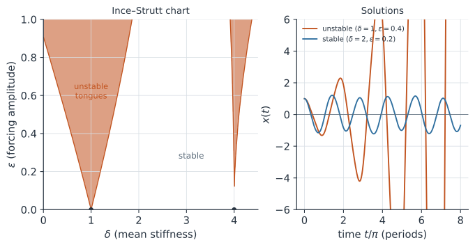
The canonical test case is the Mathieu equation, a mass on a spring whose stiffness is modulated periodically, $$\ddot{x} + \big(\delta + 2\varepsilon\cos 2t\big)\,x = 0.$$ Writing $\mathbf{x} = (x, \dot x)$ puts it in first-order form with $$A(t) = \begin{bmatrix} 0 & 1 \\ -(\delta + 2\varepsilon\cos 2t) & 0 \end{bmatrix},$$ and the forcing $\cos 2t$ has period $T = \pi$. There is no elementary closed form for $\Phi(t)$, so we integrate the two columns of $\Phi$ numerically from $t = 0$ to $t = \pi$, read off $M = \Phi(\pi)$, and take its eigenvalues.

Because the equation has no damping, the system is Hamiltonian and $\det M = 1$; the two multipliers are therefore reciprocals, $\mu_1\mu_2 = 1$. That forces a clean dichotomy in terms of the trace: when $|\operatorname{tr} M| < 2$ the multipliers are a complex-conjugate pair on the unit circle (bounded, marginally stable), and when $|\operatorname{tr} M| > 2$ they are real reciprocals with one outside the circle (unstable). Taking $\delta = 2,\ \varepsilon = 0.2$ lands in a stable band, while $\delta = 1,\ \varepsilon = 0.4$ sits inside the first parametric-resonance tongue and is unstable. Sweeping the $(\delta, \varepsilon)$ plane and shading where $|\operatorname{tr} M| > 2$ reproduces the Ince–Strutt chart in the figure, with instability tongues opening from $\delta = n^2$.

In code#

R#

# Mathieu equation: monodromy matrix and Floquet multipliers.
library(deSolve)

# Variational system for the two columns of the fundamental matrix Phi.
# State is c(Phi[1,1], Phi[2,1], Phi[1,2], Phi[2,2]).
mathieu <- function(t, y, p) with(p, {
  q <- delta + 2 * eps * cos(2 * t)
  list(c(y[2], -q * y[1],      # d/dt of column 1
         y[4], -q * y[3]))     # d/dt of column 2
})

monodromy <- function(delta, eps, Tper = pi) {
  y0 <- c(1, 0, 0, 1)          # Phi(0) = I
  out <- ode(y0, c(0, Tper), mathieu, list(delta = delta, eps = eps),
             rtol = 1e-11, atol = 1e-13)
  matrix(out[2, -1], 2, 2)     # M = Phi(T), filled column-wise
}

for (case in list(c(2, 0.2), c(1, 0.4))) {
  M  <- monodromy(case[1], case[2])
  mu <- eigen(M)$values
  cat(sprintf("delta=%.1f eps=%.1f | tr=%.3f det=%.3f | rho=%.3f (%s)\n",
              case[1], case[2], sum(diag(M)), det(M), max(Mod(mu)),
              ifelse(max(Mod(mu)) > 1 + 1e-6, "unstable", "stable")))
}

Python#

import numpy as np
from scipy.integrate import solve_ivp

T = np.pi  # period of cos(2t) in the Mathieu equation

def monodromy(delta, eps):
    """Integrate the fundamental matrix Phi over one period; return M = Phi(T)."""
    def rhs(t, Y):
        q = delta + 2.0 * eps * np.cos(2.0 * t)
        A = np.array([[0.0, 1.0], [-q, 0.0]])
        return (A @ Y.reshape(2, 2)).ravel()
    sol = solve_ivp(rhs, (0.0, T), np.eye(2).ravel(),
                    rtol=1e-11, atol=1e-13)
    return sol.y[:, -1].reshape(2, 2)

for delta, eps, tag in [(2.0, 0.2, "stable band"),
                        (1.0, 0.4, "first tongue")]:
    M = monodromy(delta, eps)
    mu = np.linalg.eigvals(M)          # Floquet multipliers
    rho = np.max(np.abs(mu))           # spectral radius
    verdict = "unstable" if rho > 1 + 1e-6 else "stable (bounded)"
    print(f"delta={delta}, eps={eps} ({tag}):")
    print(f"  trace(M)={np.trace(M):+.3f}, det(M)={np.linalg.det(M):.3f}")
    print(f"  |multipliers| = {np.abs(mu)[0]:.3f}, {np.abs(mu)[1]:.3f}"
          f"  ->  spectral radius {rho:.3f} ({verdict})")

delta=2.0, eps=0.2 (stable band):
  trace(M)=-0.575, det(M)=1.000
  |multipliers| = 1.000, 1.000  ->  spectral radius 1.000 (stable (bounded))
delta=1.0, eps=0.4 (first tongue):
  trace(M)=-2.393, det(M)=1.000
  |multipliers| = 0.540, 1.853  ->  spectral radius 1.853 (unstable)

Julia#

# Mathieu equation: monodromy matrix and Floquet multipliers.
using OrdinaryDiffEq, LinearAlgebra

function fundamental!(dΦ, Φ, p, t)
    q = p.delta + 2 * p.eps * cos(2t)
    A = [0.0 1.0; -q 0.0]
    dΦ .= A * Φ
end

function monodromy(delta, eps; Tper = π)
    prob = ODEProblem(fundamental!, Matrix{Float64}(I, 2, 2),
                      (0.0, Tper), (delta = delta, eps = eps))
    sol = solve(prob, Vern9(), reltol = 1e-11, abstol = 1e-13)
    sol.u[end]                       # M = Φ(T)
end

for (delta, eps) in ((2.0, 0.2), (1.0, 0.4))
    M = monodromy(delta, eps)
    μ = eigvals(M)
    ρ = maximum(abs.(μ))
    verdict = ρ > 1 + 1e-6 ? "unstable" : "stable"
    println("delta=$delta eps=$eps | tr=$(round(tr(M), digits=3)) ",
            "det=$(round(det(M), digits=3)) | ρ=$(round(ρ, digits=3)) ($verdict)")
end

The two runs bracket the stability boundary: the stable-band case keeps both multipliers on the unit circle (spectral radius $1$, so perturbations neither grow nor decay), while the tongue case pushes one multiplier out to about $1.85$, so a disturbance grows by that factor every half-period of the drive. The determinant returning $1$ in both cases is the Hamiltonian check that the integration conserved phase-space area.

A simpler example: a seasonally forced contact rate#

The Mathieu equation needed numerical integration because its two modes mix; the scalar case that most epidemiologists meet first has a closed form. Take a directly transmitted infection whose transmission rate is seasonally forced, $$\beta(t) = \beta_0\left(1 + \varepsilon\cos\frac{2\pi t}{T}\right),$$ and ask whether it can invade a fully susceptible population. Near the disease-free state $S \approx 1$, the infected class obeys a single linear equation with a periodic coefficient, $$\frac{dI}{dt} = \big(\beta(t) - \gamma\big)\,I.$$ This is Floquet theory in one dimension, and a scalar linear ODE integrates directly: the fundamental solution is $$\Phi(t) = \exp\!\int_0^t \big(\beta(s) - \gamma\big)\,ds,$$ so the monodromy “matrix” is the number $$M = \Phi(T) = \exp\!\int_0^T \big(\beta(s) - \gamma\big)\,ds = \exp\!\big[(\beta_0 - \gamma)\,T\big],$$ because the seasonal term integrates to zero over a full period, $\int_0^T \cos(2\pi s/T)\,ds = 0$. The single Floquet multiplier is $\mu = e^{(\beta_0 - \gamma)T}$ and the Floquet exponent is $\rho = \beta_0 - \gamma$, the mean growth rate. Invasion ($\mu > 1$) therefore happens exactly when $\beta_0 > \gamma$, that is when the time-averaged $R_0 = \beta_0/\gamma$ exceeds one.

The instructive part is what drops out: the forcing amplitude $\varepsilon$ reshapes the periodic factor $P(t)$ — the growth rate genuinely waxes and wanes within the year, and for large $\varepsilon$ it goes negative for part of it — yet $\varepsilon$ cancels from the multiplier entirely. For a scalar periodic rate, only the mean of the coefficient matters. This clean averaging is special to one dimension: once the susceptible pool $S(t)$ itself cycles at an endemic state, the linearization becomes genuinely multidimensional, its coefficient matrices no longer commute across the period, and the seasonal amplitude does move the dominant multiplier — which is why the naive time-averaged $R_0$ can mislead for a fully forced endemic model.

R#

beta0 <- 0.25; gamma <- 0.20; Tper <- 365   # mean R0 = beta0/gamma = 1.25
grid <- seq(0, Tper, length.out = 2e5 + 1)

floquet <- function(eps) {
  rate <- beta0 * (1 + eps * cos(2 * pi * grid / Tper)) - gamma
  integral <- sum((rate[-1] + rate[-length(rate)]) / 2 * diff(grid))  # trapezoid
  c(exponent = integral / Tper, multiplier = exp(integral))
}

sapply(c(0, 0.3, 0.6), floquet)   # exponent is 0.05/day whatever the amplitude

Python#

import numpy as np

beta0 = 0.25      # mean transmission rate (per day)
gamma = 0.20      # recovery rate (per day); mean R0 = beta0/gamma = 1.25
T     = 365.0     # forcing period (days)

t = np.linspace(0.0, T, 200_001)   # one period on a fine grid

def growth_rate(t, eps):           # linearized rate near the disease-free state
    beta = beta0 * (1.0 + eps * np.cos(2 * np.pi * t / T))
    return beta - gamma

for eps in (0.0, 0.3, 0.6):
    integral = np.trapezoid(growth_rate(t, eps), t)   # int (beta(t)-gamma) dt
    rho = integral / T                                # Floquet exponent (per day)
    mult = np.exp(integral)                           # multiplier over one year
    print(f"eps={eps}: Floquet exponent {rho:+.5f}/day, "
          f"annual multiplier {mult:.3e}")
print(f"closed form: exponent {beta0 - gamma:+.5f}/day = mean(beta) - gamma")

eps=0.0: Floquet exponent +0.05000/day, annual multiplier 8.431e+07
eps=0.3: Floquet exponent +0.05000/day, annual multiplier 8.431e+07
eps=0.6: Floquet exponent +0.05000/day, annual multiplier 8.431e+07
closed form: exponent +0.05000/day = mean(beta) - gamma

Julia#

beta0, gamma, Tper = 0.25, 0.20, 365.0    # mean R0 = beta0/gamma = 1.25
grid = range(0, Tper; length = 200_001)

function floquet(eps)
    rate = @. beta0 * (1 + eps * cos(2π * grid / Tper)) - gamma
    integral = sum((rate[2:end] .+ rate[1:end-1]) ./ 2 .* diff(grid))  # trapezoid
    (exponent = integral / Tper, multiplier = exp(integral))
end

floquet.((0.0, 0.3, 0.6))   # exponent 0.05/day for every forcing amplitude

All three amplitudes return the same Floquet exponent, $0.05\ \text{day}^{-1}$, and the same annual multiplier: the seasonal wiggle averages out of the scalar invasion criterion even though it dominates the within-year timing of cases.

Why it matters#

Floquet theory is the tool that lets stability analysis follow a system into a periodic world. The stability of a seasonally forced disease-free state, and thus a proper time-varying reproduction number, is a Floquet-multiplier calculation on the linearization about the periodic solution rather than an eigenvalue calculation on a frozen Jacobian: the pathogen invades when the dominant multiplier of the seasonal system exceeds one, which is not the same as the time-averaged $R_0$ exceeding one. The same machinery decides whether the limit cycles of predator–prey and other oscillating models are stable, underlies the parametric-resonance instabilities that make a periodically driven system blow up at drive frequencies where the static system is perfectly stable, and connects to the period-doubling route to chaos, where a multiplier leaving the unit circle through $-1$ marks each successive bifurcation. Whenever the coefficients breathe with a period, the monodromy matrix is where stability lives.

Related#

• Equilibria and Linear Stability
• Eigenvalues and Eigenvectors
• Jacobians
• Bifurcations
• Climate Forcing in Transmission Models
• Lotka–Volterra Predator–Prey Dynamics
• Quantitative Methods