Integrals

An integral accumulates a quantity — most visually, the area under a curve. In epidemiology it is everywhere: the total number of cases over an outbreak is the area under the incidence curve, so cumulative incidence $= \int \text{incidence}\,dt$ . In probability it is equally indispensable: the area under a density is a probability, the total area is $1$ , and an expected value is an integral.

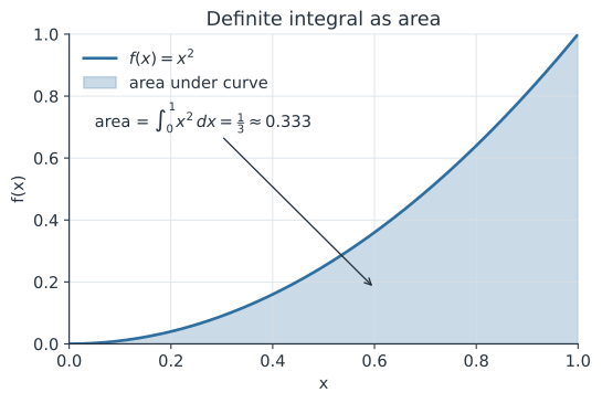
Figure 1. The definite integral as the shaded area under the curve.

Area under a curve#

The definite integral of $f$ from $a$ to $b$ is the (signed) area between the graph of $f$ and the $x$ -axis:

$\int_a^b f(x)\,dx .$

It is defined as a limit of Riemann sums — slice $[a,b]$ into $n$ pieces of width $\Delta x = (b-a)/n$ , sum the rectangle areas, and let $n \to \infty$ :

$\int_a^b f(x)\,dx = \lim_{n \to \infty} \sum_{i=1}^{n} f(x_i)\,\Delta x .$

Definite vs. indefinite#

A definite integral $\int_a^b f(x)\,dx$ is a number (an area).
An indefinite integral $\int f(x)\,dx = F(x) + C$ is a function: the family of antiderivatives of $f$ , meaning $F'(x) = f(x)$ . The constant $C$ appears because adding a constant does not change the derivative.

The Fundamental Theorem of Calculus#

The FTC links the two operations of calculus. If $F$ is any antiderivative of $f$ (so $F' = f$ ), then

$\int_a^b f(x)\,dx = F(b) - F(a) .$

In words: integration and differentiation are inverse processes. To find an area, find an antiderivative and evaluate it at the endpoints.

Worked example#

Compute $\displaystyle\int_0^1 x^2\,dx$ . An antiderivative of $x^2$ is $F(x) = \tfrac{1}{3}x^3$ (check: $F'(x) = x^2$ ). By the FTC,

$\int_0^1 x^2\,dx = F(1) - F(0) = \frac{1^3}{3} - \frac{0^3}{3} = \frac{1}{3} \approx 0.3333 .$

Computing it#

R#

# Numeric integration with base R
f <- function(x) x^2
integrate(f, lower = 0, upper = 1)
# 0.3333333 with absolute error < 3.7e-15

Python#

Python

from scipy.integrate import quad
import sympy as sp

val, err = quad(lambda x: x**2, 0, 1)
print(val)            # 0.33333333333333337

# Symbolic
x = sp.symbols("x")
print(sp.integrate(x**2, (x, 0, 1)))   # 1/3

0.33333333333333337
1/3

Julia#

Julia

using QuadGK
val, err = quadgk(x -> x^2, 0, 1)
println(val)          # 0.3333333333333333

Why it matters for statistics#

A continuous random variable $X$ has a probability density $f$ . Probabilities, the normalization condition, and the expected value are all integrals:

$P(a \le X \le b) = \int_a^b f(x)\,dx, \qquad \int_{-\infty}^{\infty} f(x)\,dx = 1, \qquad E[X] = \int_{-\infty}^{\infty} x\,f(x)\,dx .$

The cumulative distribution function $F(x) = \int_{-\infty}^{x} f(t)\,dt$ is exactly an antiderivative of the density, so by the FTC $F'(x) = f(x)$ . The same accumulation logic drives pharmacology: a drug’s total exposure (the AUC) is the integral of its concentration–time curve, $\text{AUC} = \int_0^\infty C(t)\,dt$ .