Kin Selection and Inclusive Fitness

Why would an organism pay a cost to help another reproduce? Kin selection answers that a gene for helping can spread if the help falls often enough on others who carry the same gene, so that copies gained through relatives outweigh copies lost to the helper’s own reduced success. Hamilton’s rule makes this precise, and it falls straight out of the Price equation, making this the bridge between that covariance algebra and the evolution of cooperation.

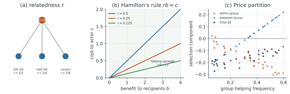
Relatedness is a regression, not a pedigree

The relatedness $r$ in kin selection is not primarily a pedigree fraction; it is a statistical regression of the recipient’s genotype on the actor’s genotype,

$$r = \frac{\operatorname{Cov}(z_{\text{recipient}}, z_{\text{actor}})}{\operatorname{Var}(z_{\text{actor}})}.$$

It measures how much extra helping genotype a recipient carries, on average, for each unit of helping genotype in the actor. Pedigree values (full sibs $\tfrac{1}{2}$, half sibs $\tfrac{1}{4}$, cousins $\tfrac{1}{8}$) are the special case where the correlation comes entirely from recent common descent, but the same regression captures relatedness generated by limited dispersal, kin recognition, or any process that clusters like genotypes together. Hamilton (1964, Journal of Theoretical Biology 7:1-52) introduced this shift from bodies to genes, and Queller (1992, American Naturalist 139:540-558, doi:10.1086/285343) showed that the regression definition is what makes the rule exact.

Hamilton’s rule from the Price equation

The Price equation partitions the change in a mean trait $\bar z$ into a selection term and a transmission term,

$$\bar w\, \Delta \bar z = \operatorname{Cov}(w_i, z_i) + \mathbb{E}(w_i\, \Delta z_i).$$

Ignore the transmission term (faithful inheritance) and write an actor’s fitness as a baseline plus a cost for its own helping and a benefit from the helping of its social partners,

$$w_i = w_0 - c\, z_i + b\, z_{-i},$$

where $z_{-i}$ is the mean helping genotype of the actor’s neighbours, $c$ the cost, and $b$ the benefit. Substituting into the covariance and using bilinearity,

$$\operatorname{Cov}(w_i, z_i) = -c\,\operatorname{Var}(z_i) + b\,\operatorname{Cov}(z_{-i}, z_i).$$

Divide through by $\operatorname{Var}(z_i)$ and recognize the relatedness regression $r = \operatorname{Cov}(z_{-i}, z_i)/\operatorname{Var}(z_i)$. The mean helping trait increases exactly when this covariance is positive, which gives Hamilton’s rule,

$$r\,b - c > 0 \quad\Longleftrightarrow\quad r\,b > c.$$

The derivation is exact for the additive fitness model and needs no approximation; the biology enters only through how $b$, $c$, and $r$ are measured.

Inclusive fitness and neighbour-modulated fitness

There are two equivalent ways to keep the books. Inclusive fitness assigns to the actor all the fitness effects its behaviour causes, weighting each recipient’s benefit by relatedness: the actor “owns” $-c + r b$. Neighbour-modulated fitness instead assigns to each individual the effects it receives from others, and averages over the population. Queller (1992) showed the two schemes give the same condition because they are two orderings of the same sum of effects, so $rb > c$ holds whichever ledger you keep.

Multilevel selection is the same accounting

The Price equation can also be expanded hierarchically: total change splits into a between-group component (selection among groups differing in mean helping) and a within-group component (selection among individuals inside groups),

$$\bar w\, \Delta \bar z = \underbrace{\operatorname{Cov}(w_g, z_g)}_{\text{between groups}} + \underbrace{\mathbb{E}\!\left[\operatorname{Cov}(w_i, z_i \mid g)\right]}_{\text{within groups}}.$$

Helping raises group productivity but is locally costly, so the between-group term is positive and the within-group term is negative, and the allele spreads when the between-group advantage wins. This multilevel partition is algebraically equivalent to the kin-selection view: high relatedness is exactly what makes between-group variance large relative to within-group variance. The same logic underlies greenbeard genes (helping directed at carriers of a recognizable marker rather than kin) and the selection for reduced virulence in spatially structured host populations, where a pathogen lineage that overexploits its local host patch harms relatives sharing that patch (Frank 1998, Foundations of Social Evolution, Princeton).

A worked example

Simulate an island model of $G = 4000$ groups with $n = 8$ individuals each, where limited dispersal makes each group cohere at its own helping frequency, generating positive relatedness. Measuring relatedness as the regression slope of group-mates’ mean genotype on an individual’s own genotype gives $r \approx 0.199$. With benefit $b = 0.6$ and cost $c = 0.08$, Hamilton’s rule reads $rb - c \approx 0.199 \times 0.6 - 0.08 \approx 0.039 > 0$, so helping should spread, and the sign of the realized selection covariance $\operatorname{Cov}(w, z) > 0$ agrees.

In code

We simulate the structured population, estimate relatedness as a regression slope, evaluate $rb - c$, and check that its sign matches the sign of the selection covariance.

R

set.seed(1834)
G <- 4000; n <- 8; b <- 0.6; c <- 0.08

p_g <- rbeta(G, 1, 3)                       # each group's helping frequency
z <- matrix(runif(G * n) < rep(p_g, each = n), G, n, byrow = TRUE) + 0
others <- (rowSums(z) - z) / (n - 1)        # mean genotype of group-mates

r <- cov(c(z), c(others)) / var(c(z))       # relatedness as a slope
w <- 1 - c * z + b * others                 # cost of own help, benefit of theirs
c(r = r, hamilton = r * b - c, cov_wz = cov(c(w), c(z)))

Python

import numpy as np

rng = np.random.default_rng(1834)
G, n = 4000, 8                     # groups, individuals per group
b, c = 0.6, 0.08                   # benefit to group-mates, cost to actor

# Limited dispersal: each group founded at its own helping frequency p_g,
# so group-mates are correlated -> positive relatedness.
p_g = rng.beta(1.0, 3.0, G)
z = (rng.random((G, n)) < p_g[:, None]).astype(float)

# Relatedness r = regression slope of group-mates' mean genotype on own.
others = (z.sum(1, keepdims=True) - z) / (n - 1)
zc, oc = z.ravel() - z.mean(), others.ravel() - others.mean()
r = np.sum(zc * oc) / np.sum(zc * zc)

# Fitness: pay cost for own helping, receive benefit from group-mates' helping.
w = 1.0 - c * z + b * others
delta = np.cov(w.ravel(), z.ravel(), bias=True)[0, 1]   # sign of Cov(w, z)

print("relatedness r =", round(r, 3))
print("Hamilton rb - c =", round(r * b - c, 4))
print("Cov(w, z) =", round(delta, 5))
print("signs agree:", np.sign(r * b - c) == np.sign(delta))

relatedness r = 0.199
Hamilton rb - c = 0.0393
Cov(w, z) = 0.00744
signs agree: True

Julia

using Random, Statistics, Distributions

Random.seed!(1834)
G, n, b, c = 4000, 8, 0.6, 0.08

p_g = rand(Beta(1, 3), G)                        # each group's helping frequency
z = Float64.(rand(G, n) .< p_g)                  # genotypes, correlated in groups
others = (sum(z, dims = 2) .- z) ./ (n - 1)

r = cov(vec(z), vec(others)) / var(vec(z))       # relatedness as a slope
w = 1 .- c .* z .+ b .* others
(r = r, hamilton = r * b - c, cov_wz = cov(vec(w), vec(z)))

Why it matters

Hamilton’s rule turns a vague appeal to “the good of the group” into a testable inequality: measure the cost, the benefit, and the relatedness, and you predict whether a social trait spreads. For infectious disease it explains why pathogens in structured host populations can evolve prudent exploitation, since overexploiting a local host harms the neighbouring parasite kin who depend on the same host, linking directly to the evolution of virulence. Because the rule is a repackaging of the Price equation, it inherits that equation’s exactness, and it makes the kin-selection and multilevel-selection accounts of the evolution of cooperation two views of one calculation.

Related

• The Price Equation and Evolutionary Epidemiology
• The Evolution of Cooperation
• Adaptive Dynamics and the Evolution of Virulence
• Quantitative Methods