Lebesgue Integration

The Riemann integral you meet first slices the domain into thin vertical strips and adds up their areas. Lebesgue integration slices the range instead: it asks, for each height $t$, how large is the set of points where the function is at least $t$, and sums those level sets. That one change of viewpoint buys an enormous amount — a definition that works for badly behaved functions, integrates against any measure (continuous, discrete, or a mixture of the two), and provides the rigorous foundation for all of probability and expectation.

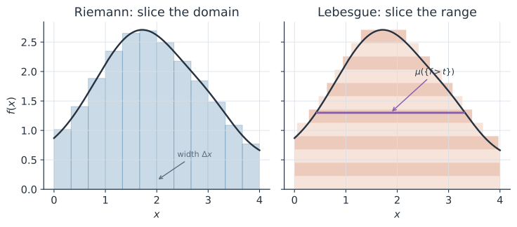
Two ways to add up a function#

Henri Lebesgue described the difference with a shopkeeper counting a pile of coins. Riemann counts them in the order he picks them up — one strip of the domain at a time. Lebesgue first sorts the coins by denomination and counts each denomination in bulk — one level of the range at a time (Figure 1). For a non-negative function the two give the same total when both make sense, and the Lebesgue recipe is captured by the layer-cake formula:

$$\int_X f \, d\mu = \int_0^\infty \mu\big(\{x : f(x) > t\}\big)\, dt . \tag{1}$$

The inner quantity $\mu(\{f>t\})$ is the “width” of the horizontal slice at height $t$ — how much of the space, as measured by $\mu$, sits above that level. Integrating those widths over all heights $t$ rebuilds the integral from its range.

Measures, and what “size” means#

A measure $\mu$ is just a consistent way of assigning a non-negative size to sets: length on the line, area in the plane, or probability on a sample space. The Lebesgue integral is defined in three steps. First, for a simple function $s = \sum_i c_i \mathbf{1}_{A_i}$ (a finite sum of constant values $c_i$ on disjoint sets $A_i$), the integral is the obvious weighted total $\int s\, d\mu = \sum_i c_i\, \mu(A_i)$. Second, for a non-negative $f$, the integral is the supremum of $\int s\, d\mu$ over all simple $s \le f$ — you approximate from below by ever-finer horizontal layers. Third, a signed function is split into its positive and negative parts $f = f^+ - f^-$, and $f$ is integrable when $\int |f|\, d\mu < \infty$.

Sets of measure zero don’t matter#

Because the integral is built from the sizes of sets, anything happening on a set of measure zero is invisible to it. Two functions that agree almost everywhere — everywhere except a set of measure zero — have the same integral. The textbook illustration is the Dirichlet function, the indicator of the rationals $\mathbf{1}_{\mathbb{Q}}$ on $[0,1]$: it jumps between $0$ and $1$ so wildly that no Riemann sum converges, yet its Lebesgue integral is simply $0$, because the rationals are countable and hence have measure zero. The same principle is quietly reassuring in epidemiology: the exact instants at which infections occur form a measure-zero set of time points, so redefining a hazard on an isolated instant cannot change anyone’s cumulative risk.

The layer cake and mean time-to-event#

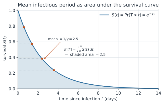
The layer-cake formula is not an abstraction you file away — it is the identity behind one of the most used facts in survival analysis. Take $\mu$ to be a probability and $f$ the value of a non-negative random variable $T$ (say, the duration of infectiousness). Then $\mu(\{T > t\})$ is exactly the survival function $S(t) = \Pr(T > t)$, and (1) becomes

$$\mathbb{E}[T] = \int_0^\infty S(t)\, dt . \tag{2}$$

The mean of a non-negative variable is the area under its survival curve. If the infectious period is exponential with clearance rate $\gamma$, then $S(t) = e^{-\gamma t}$, and (2) gives $\mathbb{E}[T] = \int_0^\infty e^{-\gamma t}\, dt = 1/\gamma$ — the familiar mean duration, read straight off the survival curve.

A funky scenario: infection pressure with superspreading atoms#

Here is where slicing the range earns its keep. Track the cumulative force of infection on a patient — the accumulated hazard $\Lambda((0,t])$ they have been exposed to by time $t$ — in a world with two very different exposure channels. There is a steady, diffuse background: everyday community contact contributes hazard at a smooth rate $\lambda(s)$. And there are superspreading events: a crowded ward round, a choir practice, a poorly ventilated ICU bay — each a single instant that dumps a discrete lump $a_k$ of infection pressure all at once.

The natural object is a measure $\Lambda$ that is part absolutely continuous (the background) and part atomic (the point masses at event times $\tau_k$):

$$\Lambda\big((0,t]\big) = \underbrace{\int_0^t \lambda(s)\, ds}_{\text{continuous background}} \;+\; \underbrace{\sum_{k:\, \tau_k \le t} a_k}_{\text{superspreading atoms}} . \tag{3}$$

A pure Riemann integral cannot express the second term — a point mass sits on a set of length zero, so a $\int (\cdot)\, dt$ never sees it. The Lebesgue (more precisely Lebesgue–Stieltjes) integral against $\Lambda$ handles both with a single definition: the continuous part integrates as usual, and each atom contributes $a_k$ exactly, so “sum” and “integral” are two faces of one operation. The probability of still being uncolonized is the survival curve $S(t) = \exp\!\big(-\Lambda((0,t])\big)$, which decays smoothly during quiet stretches and drops in a step at every superspreading event.

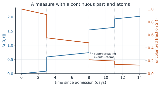
The same trick — one integral over a mixed measure — is exactly what you need whenever a quantity is neither purely continuous nor purely discrete. An infectious dose distribution with an atom at zero (most contacts transmit nothing) plus a continuous tail (a few deliver a real dose) has $\mathbb{E}[g(D)] = \int g\, d\mu$ in one stroke, with no need to bolt a sum onto an integral by hand.

Swapping limits and integrals#

One more payoff makes Lebesgue integration indispensable in computation. The dominated convergence theorem says that if $f_n \to f$ pointwise and all the $f_n$ are bounded by one integrable function $g$, then $\lim_n \int f_n\, d\mu = \int f\, d\mu$ — you may pass the limit inside the integral. This is the license behind Monte Carlo: the sample average of a simulated estimator converges to the true expectation, an integral against the model’s probability measure. It is also what lets you differentiate under the integral sign when fitting models, and it is far cleaner to state and use in the Lebesgue framework than the Riemann one.

In code#

The two blocks below compute the mean infectious period by the layer-cake identity (2) and evaluate the mixed-measure survival (3).

R#

# Mean infectious period as the area under the survival curve: E[T] = ∫ S dt
gamma <- 0.4
S <- function(t) exp(-gamma * t)
integrate(S, 0, Inf)$value      # 2.5, matching 1/gamma
1 / gamma

# Mixed measure: continuous background hazard + superspreading atoms
lam0  <- 0.03
atoms <- list(c(3, 0.5), c(8, 0.8), c(11, 0.3))   # (time, jump)
Lambda <- function(t) lam0 * t + sum(sapply(atoms, function(a) a[2] * (a[1] <= t)))
for (t in c(2, 5, 10, 14))
  cat(t, round(Lambda(t), 3), round(exp(-Lambda(t)), 3), "\n")

Python#

import numpy as np
from scipy.integrate import quad

# Mean infectious period via the layer-cake identity  E[T] = ∫ S(t) dt
gamma = 0.4
S = lambda t: np.exp(-gamma * t)             # survival of the infectious period
mean_layercake, _ = quad(S, 0, np.inf)
print(round(mean_layercake, 6), round(1 / gamma, 6))   # layer cake vs 1/gamma

# A measure with a continuous part plus atoms (superspreading events)
lam0 = 0.03                                   # continuous background hazard / day
atoms = [(3.0, 0.5), (8.0, 0.8), (11.0, 0.3)]  # (time, jump)
def Lambda(t):
    return lam0 * t + sum(a for (tau, a) in atoms if tau <= t)

for t in (2.0, 5.0, 10.0, 14.0):
    print(t, round(Lambda(t), 3), round(np.exp(-Lambda(t)), 3))   # t, Lambda, survival

2.5 2.5
2.0 0.06 0.942
5.0 0.65 0.522
10.0 1.6 0.202
14.0 2.02 0.133

The first line printed above, 2.5 2.5, is the layer-cake identity at work: the code integrates the survival curve $S(t) = e^{-\gamma t}$ and gets the same $1/\gamma = 2.5$ days as the closed form. Figure 3 shows exactly what that quad call accumulates — the shaded area under the survival curve is the mean infectious period, and each height $t$ contributes the level-set measure $\mu(\{T>t\}) = S(t)$.

Julia#

using QuadGK

# Mean infectious period as the area under the survival curve
gamma = 0.4
S(t) = exp(-gamma * t)
mean_layercake, _ = quadgk(S, 0, Inf)       # 2.5 = 1/gamma
println(mean_layercake, "  ", 1 / gamma)

# Mixed measure: continuous background + superspreading atoms
lam0  = 0.03
atoms = [(3.0, 0.5), (8.0, 0.8), (11.0, 0.3)]
Lambda(t) = lam0 * t + sum(a for (tau, a) in atoms if tau <= t; init = 0.0)
for t in (2.0, 5.0, 10.0, 14.0)
    println(t, "  ", round(Lambda(t); digits = 3), "  ", round(exp(-Lambda(t)); digits = 3))
end

Why it matters#

Modern probability is measure theory: a probability is a measure of total mass one, a random variable is a measurable function, and an expected value is a Lebesgue integral against the probability measure. That single definition covers discrete variables (integration against a counting measure is a sum), continuous ones (integration against a density recovers the ordinary integral), and the mixed cases that pervade infectious-disease data — doses with an atom at zero, hazards punctuated by superspreading events, counting processes built from Lebesgue–Stieltjes integrals. You rarely construct these integrals by hand, but the framework is what makes expectations, survival functions, and the convergence of your simulations rest on solid ground.

Related#

• Integrals
• Expected Value
• Random Variables
• Survival Analysis
• The Renewal Equation
• Quantitative Methods