Linkage Disequilibrium

Linkage disequilibrium (LD) is the non-random association of alleles at different loci — knowing the allele carried at one site tells you something about the allele at another. Basically, some genes are more “stuck” to eachother than others (e.g., they are more likely to travel together on a loci than be randomly disperse among others). It is what lets a genotyping chip “tag” millions of untyped variants with a few hundred thousand markers, and it is the reason a genetic association can point near, but not exactly at, the causal variant.

Defining the association#

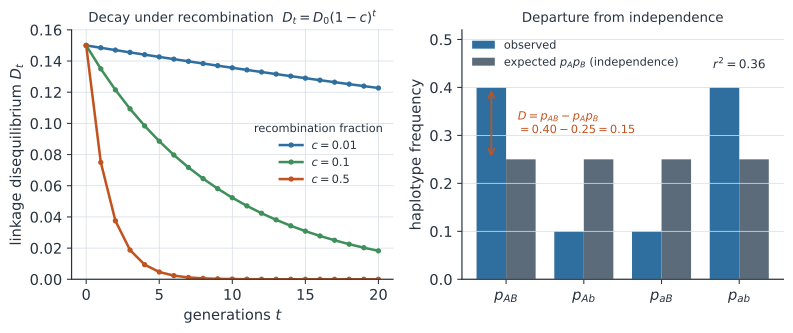
Consider two biallelic loci with alleles $A/a$ at the first and $B/b$ at the second. Let $p_A$ and $p_B$ be the allele frequencies and $p_{AB}$ the frequency of the haplotype carrying both $A$ and $B$. If the alleles were associated at random, we would expect $p_{AB} = p_A p_B$. The coefficient of linkage disequilibrium measures the departure from that independence: $$D = p_{AB} - p_A p_B .$$ When $D = 0$ the loci are in linkage equilibrium; the sign and size of $D$ capture the direction and strength of the association, much like a covariance between the two alleles treated as $0/1$ random variables.

Normalized measures#

The raw $D$ is hard to compare across loci because its range depends on the allele frequencies. Lewontin’s $D'$ rescales by the maximum value $D$ could take given those frequencies: $$D' = \frac{D}{D_{\max}}, \qquad D_{\max} = \begin{cases} \min(p_A p_b,\; p_a p_B) & D > 0,\\[2pt] \min(p_A p_B,\; p_a p_b) & D < 0, \end{cases}$$ where $p_a = 1 - p_A$ and $p_b = 1 - p_B$. The most widely used measure is the squared correlation coefficient between the two loci: $$r^2 = \frac{D^2}{p_A\, p_a\, p_B\, p_b} .$$ Here $r^2$ ranges from $0$ (independence) to $1$ (perfect correlation, where one locus perfectly predicts the other), and it is directly related to the probability of detecting an association at a tag SNP.

Decay under recombination#

Recombination breaks up haplotypes and erodes LD over the generations. If $c$ is the recombination fraction between the two loci (the probability of a crossover between them per meiosis), then the disequilibrium decays geometrically: $$D_t = D_0 (1 - c)^t .$$ Tightly linked loci (small $c$) retain LD for many generations, while unlinked loci ($c = 0.5$) lose half of any remaining $D$ each generation (Figure 1).

This decay is why LD blocks are local: over long times only nearby variants stay correlated.

Worked example#

Suppose two loci have haplotype frequencies $$p_{AB} = 0.4,\quad p_{Ab} = 0.1,\quad p_{aB} = 0.1,\quad p_{ab} = 0.4 .$$ The allele frequencies follow by summing: $$p_A = p_{AB} + p_{Ab} = 0.5, \qquad p_B = p_{AB} + p_{aB} = 0.5,$$ so $p_a = 0.5$ and $p_b = 0.5$. The disequilibrium coefficient is $$D = p_{AB} - p_A p_B = 0.4 - (0.5)(0.5) = 0.15 .$$ Because $D > 0$, $D_{\max} = \min(p_A p_b, p_a p_B) = \min(0.25, 0.25) = 0.25$, giving $D' = 0.15 / 0.25 = 0.6$. The squared correlation is $$r^2 = \frac{0.15^2}{(0.5)(0.5)(0.5)(0.5)} = \frac{0.0225}{0.0625} = 0.36 .$$ So the two loci share $36\%$ of their variation: a marker at one would capture a good deal, but not all, of an association at the other.

Why it matters in practice#

LD underpins several core methods in statistical genetics.

• Tag SNPs: because nearby variants are correlated, a genotyping array covers the genome by choosing markers in high $r^2$ with their neighbors, and imputation reconstructs untyped variants from LD patterns.
• Fine-mapping: a GWAS association signal is spread across all variants in LD with the causal one, so disentangling them requires modeling the local LD structure.
• Instrument validity: in Mendelian randomization, a genetic instrument can be invalid if it is in LD with a variant affecting the outcome through another pathway.

In code#

R#

pAB <- 0.4; pAb <- 0.1; paB <- 0.1; pab <- 0.4
pA <- pAB + pAb; pB <- pAB + paB
pa <- 1 - pA;    pb <- 1 - pB

D <- pAB - pA * pB                                  # 0.15
Dmax <- if (D > 0) min(pA * pb, pa * pB) else min(pA * pB, pa * pb)
Dprime <- D / Dmax                                  # 0.6
r2 <- D^2 / (pA * pa * pB * pb)                      # 0.36
c(D = D, Dprime = Dprime, r2 = r2)

# decay of D over 10 generations at recombination fraction c = 0.1
c_rec <- 0.1
D * (1 - c_rec)^(0:10)

Python#

pAB, pAb, paB, pab = 0.4, 0.1, 0.1, 0.4
pA = pAB + pAb; pB = pAB + paB
pa = 1 - pA;    pb = 1 - pB

D = pAB - pA * pB                                    # 0.15
Dmax = min(pA * pb, pa * pB) if D > 0 else min(pA * pB, pa * pb)
Dprime = D / Dmax                                    # 0.6
r2 = D**2 / (pA * pa * pB * pb)                       # 0.36
print(D, Dprime, r2)

c_rec = 0.1
[D * (1 - c_rec)**t for t in range(11)]              # geometric decay

0.15000000000000002 0.6000000000000001 0.3600000000000001

Julia#

pAB, pAb, paB, pab = 0.4, 0.1, 0.1, 0.4
pA = pAB + pAb; pB = pAB + paB
pa = 1 - pA;    pb = 1 - pB

D = pAB - pA * pB                                     # 0.15
Dmax = D > 0 ? min(pA*pb, pa*pB) : min(pA*pB, pa*pb)
Dprime = D / Dmax                                    # 0.6
r2 = D^2 / (pA * pa * pB * pb)                        # 0.36
println((D, Dprime, r2))

c_rec = 0.1
[D * (1 - c_rec)^t for t in 0:10]                    # decay over generations

Why it matters#

Linkage disequilibrium is the statistical glue between genotype and phenotype maps. Its magnitude decides how densely we must genotype, how precisely we can localize a causal variant, and whether a genetic instrument is clean — so quantifying $D$, $D'$, and especially $r^2$ is a prerequisite for interpreting essentially any modern association study.

Related#

• Hardy–Weinberg Equilibrium
• GWAS
• Population Stratification
• Mendelian Randomization
• Instrumental Variables
• Random Variables
• Quantitative Methods