Multilevel Regression and Poststratification
Surveys are rarely representative of the population you care about, and the subgroups you most want estimates for — a single county, a narrow age band, a small demographic cell — are exactly the ones with too few respondents to estimate directly. Multilevel regression and poststratification (MRP) solves both problems at once: it fits a multilevel model that borrows strength across cells to stabilize sparse estimates, then reweights those cell estimates by known population totals so the result reflects the actual population rather than the sample (Downes & Carlin 2019, doi:10.1002/bimj.201900023). It has become a standard tool for small-area estimation of disease prevalence and health behaviors.
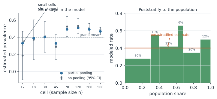
The two steps#
MRP is exactly what its name lists, in order.
Multilevel regression. Model the outcome — say, whether a respondent has a condition — as a function of demographic and geographic predictors, entering categorical variables like age, race, and area as modeled (random) effects rather than fixed effects. This produces a predicted rate for every poststratification cell, defined by the cross-classification of all those predictors (for example, a 40–49-year-old woman of a given race in a given county).
Poststratification. Weight each cell’s modeled rate by the number of people in that cell in the population, from a source like the census, and sum to get an estimate for the whole population or any subpopulation,
where is the modeled rate in cell , its population size, and the target area or subgroup.
Why partial pooling is the key#
The reason to use a multilevel model rather than separate estimates per cell is partial pooling. A no-pooling estimate takes each cell’s raw sample mean, which is hopelessly noisy for small cells; a complete-pooling estimate ignores cell differences entirely. The multilevel model sits between them, shrinking each cell toward the grand mean by an amount set by the data: cells with many respondents stay near their own mean, while sparse cells borrow strength from demographically similar cells and shrink more. That is the left panel of the figure, and it is what lets MRP produce usable estimates for cells that a direct survey estimate could never support. The counterpart is that a strong geographic predictor is close to a necessary condition for MRP to perform well, because the model needs a way to distinguish areas beyond their raw sample.
Poststratification needs population totals#
The poststratification step is only as good as the population counts . These come from external population data — most often census or American Community Survey tables — cross-classified by the same variables used in the model. This is the constraint that limits how many predictors can define the cells: you can only poststratify on variables for which you have population totals, which is why MRP cells are usually built from a few demographic and geographic variables rather than a rich covariate set. When the joint population table is unavailable, variants such as poststratification from the marginal distributions extend the method to settings without a full cross-tabulation.
A worked example#
Suppose a multilevel model has produced a prevalence estimate for each of four demographic-geographic cells, and the census gives each cell’s population share. The raw survey (unweighted) mean over-represents some cells; poststratification corrects it to the population.
In code#
R#
rate <- c(0.10, 0.22, 0.15, 0.30)   # modeled prevalence per cell
pop  <- c(4000, 1000, 3000, 2000)   # population size per cell
n    <- c(300,  40,   220,  35)     # survey respondents per cell

sample_mean <- sum(rate * n) / sum(n)         # reflects the sample
poststrat   <- sum(rate * pop) / sum(pop)      # reflects the population

c(sample_mean = sample_mean, poststratified = poststrat)
Python#
import numpy as np

rate = np.array([0.10, 0.22, 0.15, 0.30])   # modeled prevalence per cell
pop = np.array([4000, 1000, 3000, 2000])    # population size per cell
n = np.array([300, 40, 220, 35])            # survey respondents per cell

sample_mean = np.sum(rate * n) / n.sum()        # reflects the sample
poststrat = np.sum(rate * pop) / pop.sum()      # reflects the population

print(f"unweighted sample mean = {sample_mean:.3f}")
print(f"poststratified estimate = {poststrat:.3f}")
unweighted sample mean = 0.138
poststratified estimate = 0.167
Julia#
rate = [0.10, 0.22, 0.15, 0.30]   # modeled prevalence per cell
pop  = [4000, 1000, 3000, 2000]   # population size per cell
n    = [300, 40, 220, 35]         # survey respondents per cell

sample_mean = sum(rate .* n) / sum(n)      # reflects the sample
poststrat   = sum(rate .* pop) / sum(pop)   # reflects the population

(sample_mean = sample_mean, poststratified = poststrat)
The two numbers differ because the small, high-prevalence cell is over-represented in the sample and down-weighted to its true population share.
Why it matters#
MRP is how a messy, non-representative survey becomes credible small-area estimates, which is why it underpins subnational maps of disease prevalence, risk behaviors, and health-care access. Its two ideas are worth separating: partial pooling makes sparse-cell estimates stable, and poststratification against population totals makes them representative. Neither alone suffices, and the method’s reach is set by which population totals you can obtain to build the cells.
Related#
- Hierarchical (Multilevel) Models — partial pooling and shrinkage
- Survey Sampling — weighting and the design-based alternative
- Areal Models and Conditional Autoregression — spatial smoothing for small areas
- Logistic Regression — the cell-level model for a binary outcome
- Bayesian Inference — the estimation framework MRP is usually fit in