Encoding Spatial Priors with VAEs (PriorVAE)

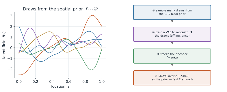
Bayesian disease mapping is slow for a frustrating reason: the prior, not the likelihood. A Gaussian-process or ICAR prior over a spatial field couples every location to every other, so each MCMC step pays for an expensive, badly-conditioned evaluation of a high-dimensional correlated prior, and the sampler mixes poorly through the resulting cramped geometry. PriorVAE, introduced by Semenova and colleagues, sidesteps this with a trick that is obvious only in hindsight: spend the cost once, offline, by training a variational autoencoder to imitate the spatial prior, then reuse its decoder — a cheap, fixed neural network — as a drop-in prior during inference. The correlated field is then generated from a handful of independent standard-normal latents, which MCMC handles beautifully.

Figure 1. Left: draws from a Gaussian-process spatial prior — smooth correlated surfaces that are costly to sample inside an MCMC loop. Right: the PriorVAE recipe — sample the prior, train a VAE to reproduce the draws offline, freeze the decoder, then run MCMC over a few independent latents that decode to the full field.

The problem PriorVAE solves#

A spatial model puts a correlated prior on a latent field $\mathbf{f} = (f_1,\dots,f_n)$ at $n$ locations or areal units, for example the Gaussian process $\mathbf{f}\sim\mathcal{N}(\mathbf{0}, K)$ with covariance $K$ , and links it to observed counts through a likelihood such as $y_i \sim \text{Poisson}(e_i\,e^{f_i})$ .

Three draws from a Gaussian-process prior over a 2D grid — smooth, spatially correlated random fields, the kind of surface a disease-mapping model places over space before seeing data. Right: the correlation between two locations decays with the distance between them, and the lengthscale sets how quickly, controlling how smooth the fields are. — Figure 2. Three draws from a Gaussian-process prior over a 2D grid — smooth, spatially correlated random fields, the kind of surface a disease-mapping model places over space before seeing data. Right: the correlation between two locations decays with the distance between them, and the lengthscale $\ell$ sets how quickly, controlling how smooth the fields are.

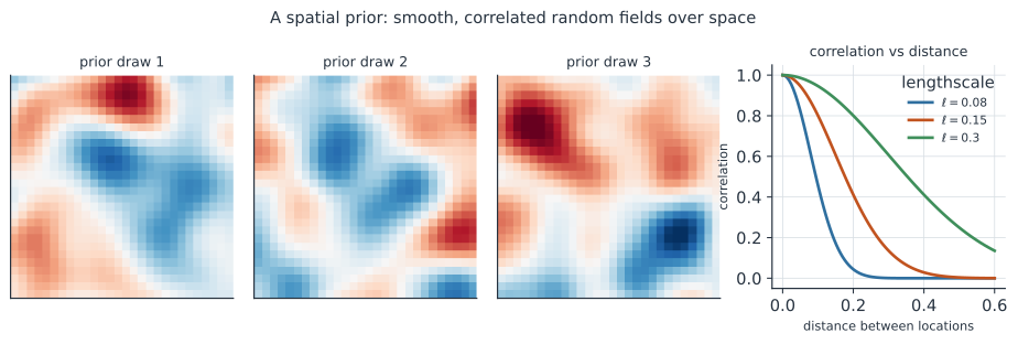
The spatial correlation in Figure 2 is the whole point of the prior — it says nearby places should have similar rates — but it is also what makes inference expensive. Two costs make this painful inside a sampler. Evaluating the prior density needs the inverse and determinant of the $n\times n$ matrix $K$ — an $\mathcal{O}(n^3)$ Cholesky at worst — repeated at every step. Worse, the strong correlations warp the posterior into a shape (a “funnel”, a thin ridge) that Hamiltonian samplers traverse slowly, so you need many steps and each step is expensive. Basis-function approximations and INLA attack the first cost; PriorVAE attacks both, and it works for priors — irregular ICAR graphs, aggregated fields, non-Gaussian processes — that those methods handle less naturally.

The PriorVAE recipe#

The method has four steps, split cleanly into an expensive offline stage and a cheap inference stage — the workflow on the right of the figure.

Sample the prior. Draw many realizations $\mathbf{f}^{(1)},\dots,\mathbf{f}^{(M)}$ from the spatial prior evaluated at the fixed set of locations you will model. This uses the slow machinery, but only once, and it is embarrassingly parallel.
Train a VAE on the draws. Fit a variational autoencoder whose “data” are these prior draws, learning an encoder $q_\phi(\mathbf{z}\mid\mathbf{f})$ and a decoder $g_\theta(\mathbf{z})\approx\mathbf{f}$ with a low-dimensional latent $\mathbf{z}\sim\mathcal{N}(\mathbf{0}, I_d)$ , $d\ll n$ . The ELBO forces the decoder to reproduce the prior’s spatial structure from a standard-normal code.
Freeze the decoder. Keep $g_\theta$ fixed. It is now a compact, differentiable surrogate for “a draw from the spatial prior”, parameterized by the independent latents $\mathbf{z}$ .
Infer over the latents. Replace the spatial prior with the decoder in the Bayesian model: put a $\mathcal{N}(\mathbf{0}, I_d)$ prior on $\mathbf{z}$ , set $\mathbf{f} = g_\theta(\mathbf{z})$ , and run MCMC. The sampler now explores an uncorrelated, low-dimensional, well-conditioned standard-normal space, and the decoder maps each proposal to a valid correlated field.

The model that goes to the sampler is simply $\mathbf{z}\sim\mathcal{N}(\mathbf{0}, I_d), \qquad \mathbf{f} = g_\theta(\mathbf{z}), \qquad y_i \sim \text{Poisson}\!\left(e_i\, e^{f_i}\right), \tag{1}$ with no $K^{-1}$ , no $\log\lvert K\rvert$ , and geometry as friendly as a standard normal.

Why a decoder can stand in for the prior#

The key fact is that the decoder learns the prior’s distribution, not one draw from it. Because the ELBO trains $g_\theta$ so that pushing a standard normal $\mathbf{z}$ through it reproduces the family of prior samples, the induced distribution of $\mathbf{f} = g_\theta(\mathbf{z})$ matches the target spatial prior — the same marginal variances and spatial correlations — up to the VAE’s approximation error. A useful special case makes this concrete and is worth running: if the decoder is linear, $g_\theta(\mathbf{z}) = B\mathbf{z}$ , then $\mathbf{f}$ is Gaussian with covariance $BB^\top$ , and choosing $B$ from the top eigenvectors of $K$ scaled by the square roots of its eigenvalues (the truncated Karhunen–Loève expansion) makes $BB^\top\approx K$ . That linear map is a low-rank generative model of a Gaussian prior — a linear PriorVAE — and it already delivers the inference speed-up. PriorVAE’s advance is to let $g_\theta$ be nonlinear, so the same recipe works when the prior is not Gaussian: an ICAR field on an irregular county graph, a log-Gaussian Cox intensity, or a field defined on shifting administrative boundaries.

Note

Freezing the decoder fixes the prior’s hyperparameters (its lengthscale, its variance) at training time. To keep them inferable, PriorCVAE conditions the decoder on the hyperparameters, and aggVAE extends the idea to spatial aggregation and change-of-support — for instance mapping malaria prevalence across redrawn district boundaries in Kenya. The closely related πVAE encodes a stochastic-process prior over functions the same way.

A worked example#

Suppose the spatial prior is a Gaussian process on $n = 25$ points with a smooth kernel, and its Karhunen–Loève expansion shows that the first $d = 6$ components already capture almost all of the prior variance.

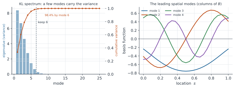
Left: the eigenvalue (Karhunen–Loève) spectrum of the prior’s covariance falls off fast, so the cumulative variance crosses about 98% by mode six. Right: those leading modes are smooth spatial basis functions — the columns of — and a draw from the prior is a weighted sum of them, so six independent coefficients encode the whole 25-dimensional correlated field. — Figure 3. Left: the eigenvalue (Karhunen–Loève) spectrum of the prior’s covariance falls off fast, so the cumulative variance crosses about 98% by mode six. Right: those leading modes are smooth spatial basis functions — the columns of $B$ — and a draw from the prior is a weighted sum of them, so six independent coefficients encode the whole 25-dimensional correlated field.

The spectrum in Figure 3 is why this works: the correlated field lives, to good approximation, in a six-dimensional subspace spanned by the leading spatial modes. Encoding the prior means keeping those six basis vectors $B\in\mathbb{R}^{25\times 6}$ ; a standard-normal $\mathbf{z}\in\mathbb{R}^6$ then decodes to a full 25-dimensional field $\mathbf{f} = B\mathbf{z}$ whose covariance reproduces the GP. Inference that would have sampled a correlated 25-dimensional field now samples six independent unit normals, so the posterior geometry is a plain sphere and the sampler mixes fast — the payoff PriorVAE brings to the far larger fields (hundreds to thousands of areal units) of real disease maps.

In code#

Python#

The runnable version uses a linear decoder — the Karhunen–Loève special case — so it executes here with numpyro, while faithfully showing PriorVAE’s inference stage: sample the prior, encode it into a low-dimensional basis, then run MCMC over independent latents that decode to the field.

Python

import numpy as np, jax, jax.numpy as jnp
import numpyro, numpyro.distributions as dist
from numpyro.infer import MCMC, NUTS
numpyro.set_host_device_count(1)
rng = np.random.default_rng(0)

s = np.linspace(0, 1, 25)                                    # spatial locations
K = np.exp(-0.5 * (s[:, None] - s[None, :]) ** 2 / 0.15 ** 2) + 1e-6 * np.eye(25)
vals, vecs = np.linalg.eigh(K)                              # "encode" the GP prior:
idx = np.argsort(vals)[::-1][:6]                            # keep the top 6 KL modes
B = jnp.asarray(vecs[:, idx] * np.sqrt(vals[idx]))         # decoder  f = B z,  z~N(0,I)

f_true = np.asarray(B) @ rng.standard_normal(6)            # a field to recover
y = f_true + 0.1 * rng.standard_normal(25)                 # noisy observations

def model(y):
    z = numpyro.sample("z", dist.Normal(jnp.zeros(6), 1.0))  # independent latents
    numpyro.sample("y", dist.Normal(B @ z, 0.1), obs=jnp.asarray(y))

mcmc = MCMC(NUTS(model), num_warmup=300, num_samples=300, num_chains=1,
            progress_bar=False)
mcmc.run(jax.random.PRNGKey(0), y=y)
f_hat = np.asarray(B) @ np.asarray(mcmc.get_samples()["z"]).mean(0)
print(f"sampled {6} independent latents in place of a correlated {25}-dim field")
print(f"posterior field RMSE vs truth: {np.sqrt(np.mean((f_hat - f_true) ** 2)):.3f}")

sampled 6 independent latents in place of a correlated 25-dim field
posterior field RMSE vs truth: 0.063

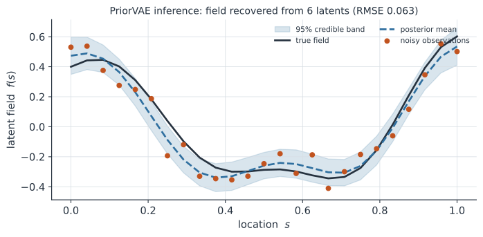
Figure 4. The output of that inference: from noisy observations, the model recovers the smooth latent field. The posterior mean tracks the true field, and the 95% credible band widens between observations and pinches where data pin it down — all from sampling six independent latents rather than a correlated 25-dimensional field.

The recovery in Figure 4 is the payoff: the posterior mean follows the truth to an RMSE of $0.063$ , with honest uncertainty everywhere, at a fraction of the sampling cost of the full correlated prior.

The full PriorVAE replaces the linear basis with a nonlinear decoder, trained offline (step 2) to reproduce draws from the spatial prior; here a small flax VAE learns the GP’s structure from 4000 draws, and its frozen decoder would then slot into the same inference model as $B$ did above:

Python

import flax.linen as fnn, optax

L = jnp.linalg.cholesky(jnp.asarray(K))              # sample the GP prior (step 1)
key = jax.random.PRNGKey(0)
draws = (L @ jax.random.normal(key, (25, 4000))).T   # 4000 draws, each a 25-dim field

class PriorVAE(fnn.Module):                           # nonlinear encoder + decoder
    @fnn.compact
    def __call__(self, x, key):
        h = fnn.tanh(fnn.Dense(32)(x))
        mu, logvar = fnn.Dense(6)(h), fnn.Dense(6)(h)
        z = mu + jnp.exp(0.5 * logvar) * jax.random.normal(key, mu.shape)
        return fnn.Dense(25)(fnn.tanh(fnn.Dense(32)(z))), mu, logvar

vae = PriorVAE()
params = vae.init(key, draws[:1], key)
opt = optax.adam(2e-3); state = opt.init(params)
def elbo_loss(p, x, k):
    xh, mu, lv = vae.apply(p, x, k)
    recon = jnp.mean(jnp.sum((xh - x) ** 2, 1))
    kl = jnp.mean(-0.5 * jnp.sum(1 + lv - mu ** 2 - jnp.exp(lv), 1))
    return recon + 0.01 * kl

@jax.jit
def train_step(p, state, x, k):
    loss, grads = jax.value_and_grad(elbo_loss)(p, x, k)
    updates, state = opt.update(grads, state)
    return optax.apply_updates(p, updates), state, loss

for _ in range(400):                                  # train the VAE offline (step 2)
    key, k = jax.random.split(key)
    params, state, loss = train_step(params, state, draws, k)
print(f"nonlinear PriorVAE trained on GP draws: reconstruction loss {float(loss):.1f}")

nonlinear PriorVAE trained on GP draws: reconstruction loss 1.0

The nonlinear decoder is what lets the same recipe handle priors the linear basis cannot — an ICAR field on an irregular graph, or an aggregated/change-of-support prior.

R#

# Train the VAE offline (torch/keras), export the decoder weights, then do the
# Bayesian inference in a probabilistic language. Here the numpyro-style model
# expressed with cmdstanr, feeding a frozen decoder as generated quantities.
library(cmdstanr)
# Stan model sketch:
#   parameters { vector[d] z; }
#   model      { z ~ std_normal();
#                y ~ poisson_log(log_expected + decoder(z)); }   // decoder = fixed NN

Julia#

Julia

# Flux to train the decoder offline; Turing.jl for inference over the latents.
using Turing, Flux
@model function priorvae(y, expected, decoder)
    z ~ MvNormal(zeros(d), I)             # independent latents
    f = decoder(z)                        # frozen VAE decoder -> spatial field
    @. y ~ Poisson(expected * exp(f))
end

Why it matters#

PriorVAE is a template for a broader move: amortize an expensive prior into a neural network so that Bayesian inference stays cheap and honest. For spatial epidemiology this means disease maps over many small areas — prevalence, incidence, mortality — with the full uncertainty quantification of a hierarchical Bayesian model but a fraction of the sampling cost, and with the flexibility to encode priors that resist closed-form treatment. More broadly it joins deep generative modelling to principled inference: the neural network does not replace the Bayesian model or invent the prior, it compresses a prior you already trust into a form the sampler likes, keeping the interpretability and calibrated uncertainty that make a model useful for public-health decisions. The same idea generalizes beyond space — to priors over time series, functions, and mechanistic-model outputs — wherever a trusted but intractable prior is the bottleneck.