Proportional Odds Models

Many outcomes are ordered but not numeric: none / mild / moderate / severe; a functional-status scale; a COVID clinical scale from discharged to ventilated to dead. The temptation is to collapse the order into a yes/no event and reach for logistic regression, but dichotomizing throws away the gradations that make an ordinal outcome informative. The proportional odds model — the most widely used ordinal-regression model — keeps every level of the outcome while still reporting a single, interpretable odds ratio.

Left: a continuous latent variable underlies the ordinal outcome, and fixed cutpoints slice it into ordered categories; a treatment shifts the whole latent distribution by the same amount on the log-odds scale, so every cutpoint sees the same shift — that shared shift is the proportional-odds assumption. Right: the shift moves probability mass toward higher categories. — Figure 1. Left: a continuous latent variable underlies the ordinal outcome, and fixed cutpoints slice it into ordered categories; a treatment shifts the whole latent distribution by the same amount $\beta$ on the log-odds scale, so every cutpoint sees the same shift — that shared shift is the proportional-odds assumption. Right: the shift moves probability mass toward higher categories.

The cumulative-logit model#

Let the outcome $Y$ take ordered values $1 < 2 < \cdots < J$ . Rather than model each category directly, the proportional odds model works with the cumulative probabilities $\Pr(Y \ge j)$ and puts each on the log-odds scale as a linear function of the predictors, $\operatorname{logit}\,\Pr(Y \ge j \mid x) = \alpha_j + x^\top\beta, \qquad j = 2,\dots,J. \tag{1}$ This is the model of McCullagh (1980), building on Walker and Duncan (1967). Two features define it:

Each cutpoint gets its own intercept $\alpha_j$ (a decreasing sequence), which sets how common the higher categories are.
The slope $\beta$ is shared across all cutpoints. There is one $\beta$ , not $J-1$ of them.

Because the slope is common, the effect of a predictor is a single number: a one-unit increase in $x_k$ multiplies the odds of being in a higher category — at every cutpoint simultaneously — by the same $\text{OR}_k = e^{\beta_k}.$ That is the “proportional odds”: the cumulative odds ratio is the same no matter where you split the scale.

Why “proportional odds” looks the way it does#

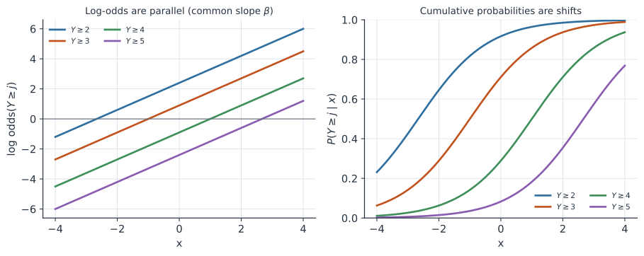
On the log-odds scale, (1) is a family of parallel lines — same slope $\beta$ , different intercepts $\alpha_j$ (Figure 2, left). On the probability scale it is a family of cumulative curves $\Pr(Y \ge j \mid x)$ that are horizontal shifts of one another (Figure 2, right).

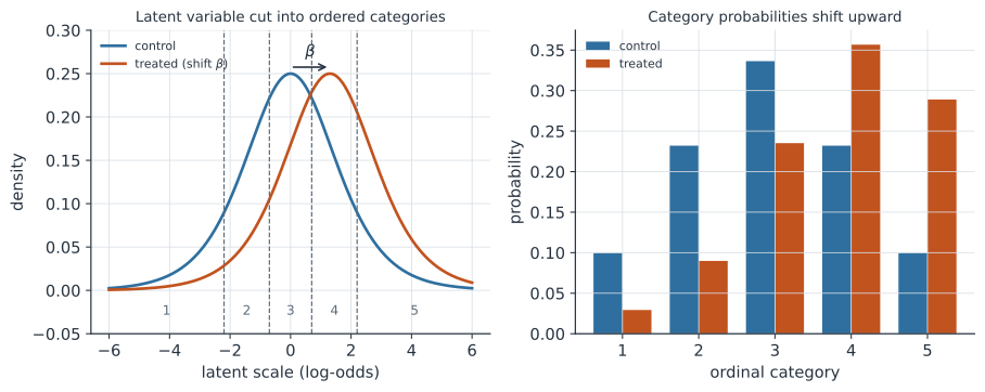
Left: the model makes linear in with the same slope for every cutpoint , so the lines are parallel. Right: on the probability scale this is a family of cumulative curves that are shifts of one another. A single odds ratio moves you the same multiplicative distance at every cutpoint. — Figure 2. Left: the model makes $\log\,\mathrm{odds}(Y \ge j)$ linear in $x$ with the same slope for every cutpoint $j$ , so the lines are parallel. Right: on the probability scale this is a family of cumulative curves that are shifts of one another. A single odds ratio moves you the same multiplicative distance at every cutpoint.

A clean way to see where the model comes from is the latent-variable view (Figure 1). Imagine an unobserved continuous severity $Y^\* = x^\top\beta + \varepsilon$ with a logistic error $\varepsilon$ , and fixed thresholds $-\alpha_2 > \cdots > -\alpha_J$ that we cross to move up categories. A predictor shifts the entire latent distribution by $x^\top\beta$ , so it moves every threshold-crossing probability by the same amount — which is exactly the equal-slopes assumption. Swap the logistic error for an extreme-value (Gumbel) distribution and you get the proportional hazards ordinal model instead (a complementary-log-log link); this is the hinge that connects the proportional odds model to survival analysis, below.

Fitting#

The category probabilities are differences of adjacent cumulative probabilities, $\Pr(Y = j \mid x) = \Pr(Y \ge j \mid x) - \Pr(Y \ge j+1 \mid x),$ and the parameters $(\alpha_2,\dots,\alpha_J,\beta)$ are estimated by maximum likelihood, just as in logistic regression. With $J=2$ categories there is a single cutpoint and (1) is ordinary binary logistic regression — the proportional odds model is its direct generalization to more than two ordered levels.

Contrast: proportional odds vs binary logistic regression#

The relationship to logistic regression is the clearest way to see what the ordinal model buys you.

It is the same family. Binary logistic regression is the proportional odds model with two categories; the ordinal model simply allows $J-1$ cutpoints tied together by one slope.
It avoids throwing away information. To use logistic regression on an ordinal outcome you must dichotomize — pick one cutpoint (e.g. “severe or worse” vs “not”) and discard the ordering on either side. Frank Harrell argues at length that this wastes information and statistical power, and that the choice of cut is arbitrary and manipulable (“Resources for Ordinal Regression Models” and “Information Gain From Using Ordinal Instead of Binary Outcomes”).
One effect instead of many. Fitting a separate logistic regression at each cutpoint would give you $J-1$ different odds ratios for the same predictor and no coherent summary; the proportional odds model reports one odds ratio that applies across the whole scale.
It handles floor and ceiling effects and ties gracefully, because it never assumes the category codes are equally spaced numbers — only that they are ordered. The model is invariant to any monotone recoding of $Y$ .

Note

When the sole predictor is a two-group indicator and there is no covariate adjustment, the proportional odds model is essentially equivalent to the Wilcoxon–Mann–Whitney rank test, and to the Kruskal–Wallis test for several groups. Frank Harrell makes this connection central: the model is a regression generalization of the Wilcoxon test, and its treatment odds ratio has an almost one-to-one relationship with the concordance probability (the probability that a randomly chosen treated subject ranks higher than a randomly chosen control), which is the Wilcoxon statistic itself (Harrell, “Resources for Ordinal Regression Models”).

Contrast: proportional odds vs survival / Cox regression#

The proportional odds model and survival analysis are close cousins, because “which ordered category” and “how long until the event” are both questions about ordered outcomes with a monotone structure.

Same machinery, different link. Modeling $\Pr(Y \ge j)$ with a logit link gives proportional odds; modeling it with a complementary-log-log link gives a grouped proportional-hazards model — the discrete-time analogue of Cox regression. The Cox model is, in effect, an ordinal model in which the “categories” are the ordered event times and the coefficients are constant across all of them, just as the ordinal slope is constant across all cutpoints.
Censoring is the practical divider. Survival models are built to handle right-censoring — subjects for whom the event has not yet happened. A standard ordinal outcome has no censoring: every subject lands in an observed category. When follow-up is complete and the outcome is an ordered status at a fixed time, an ordinal model is often simpler and more directly interpretable than a time-to-event model.
A unifying view. Harrell emphasizes that a proportional odds model with a large number of categories can even accommodate a continuous outcome, treating each distinct value as its own level — a semiparametric regression that makes no distributional assumption about $Y$ and is robust to its transformation, much as the Cox model makes none about the baseline hazard. This is the ordinal model as a general-purpose alternative to linear regression when $Y$ is skewed, bounded, or full of ties.

The through-line: logistic, proportional odds, and Cox regression are one modeling idea — a linear predictor acting on the log-odds or log-hazard of exceeding a threshold — differing in the link function and in whether the “thresholds” are outcome categories or event times.

The proportional-odds assumption — and Harrell’s “not fatal” argument#

Equation (1) assumes the odds ratio is the same at every cutpoint. This can be checked by fitting separate cutpoint-specific slopes and seeing whether they differ, by score tests, or by graphical checks — but Harrell cautions strongly against the common practice of using a significance test of the assumption to decide whether to use the model.

His position, argued in “Violation of Proportional Odds is Not Fatal” and “Assessing the Proportional Odds Assumption and Its Impact”, has several strands:

The assumption is no stronger than what competitors already assume. Dichotomizing to a binary logistic regression assumes proportional odds and discards data; a $t$ -test assumes far more.
Under mild violation the pooled odds ratio is a sensible average. When odds ratios vary across cutpoints, the single PO estimate behaves like a well-defined weighted average odds ratio, and it stays tightly linked to the concordance (Wilcoxon) probability — so it remains a meaningful, powerful summary of whether one group tends toward higher categories.
Assessment should be about impact, not $p$ -values. Better to compare the PO model’s predictions against a more flexible model (e.g. a partial proportional odds or multinomial fit) and ask whether conclusions actually change, rather than reject PO on a low-power or over-powered test.

When a specific predictor genuinely needs to escape the equal-slopes constraint, the partial proportional odds model of Peterson and Harrell (1990) relaxes the assumption for that predictor while keeping it for the rest — a targeted fix rather than abandoning the ordinal framework.

Worked example: reading an ordinal odds ratio#

A trial reports a treatment coefficient $\hat\beta = 1.3$ on a five-level ordinal recovery scale from a proportional odds model. The odds ratio is $e^{1.3} \approx 3.7$ . The interpretation is uniform across the scale: treated patients have about $3.7$ times the odds of being in a better category than control, whether “better” means “beyond the worst level,” “beyond moderate,” or “in the best level.”

There is no separate number to report per cutpoint — that single $3.7$ is the treatment effect, and via the Wilcoxon connection it corresponds (through Harrell’s approximation $\text{OR} \approx [c/(1-c)]^{1.52}$ ) to a concordance probability of roughly $0.70$ (a randomly chosen treated patient out-recovers a randomly chosen control about $70\%$ of the time). Contrast that with dichotomizing at “full recovery vs not,” which would answer a narrower question with less power and an arbitrary threshold.

In code#

R#

## Frank Harrell's rms package: orm() fits proportional odds for any number
## of levels (including effectively continuous Y), lrm() for modest J.
library(rms)
dd <- datadist(d); options(datadist = "dd")

f <- lrm(y ~ treat + age, data = d)   # y is an ordered factor
f                                     # slopes are shared across cutpoints
exp(coef(f)["treat"])                 # the single treatment odds ratio

## Assess the PO assumption by IMPACT, not just a test:
## compare predicted probabilities to a more flexible model (Harrell's advice).
impactPO(y ~ treat + age, data = d)   # PO vs multinomial/partial-PO predictions

## Base-R alternative:
library(MASS)
polr(ordered(y) ~ treat + age, data = d, Hess = TRUE)   # cumulative-logit

Python#

Python

import numpy as np
from statsmodels.miscmodels.ordinal_model import OrderedModel

rng = np.random.default_rng(0)
n = 500
x = rng.normal(size=n)
treat = rng.integers(0, 2, size=n)

# Proportional-odds data-generating process: shift a logistic latent variable,
# then cut it at fixed thresholds into 4 ordered categories.
latent = 1.0 * x + 1.3 * treat + rng.logistic(size=n)
cuts = np.quantile(latent, [0.25, 0.50, 0.75])
y = np.digitize(latent, cuts)          # ordered outcome 0,1,2,3

mod = OrderedModel(y, np.column_stack([x, treat]), distr="logit")
res = mod.fit(method="bfgs", disp=False)

b = np.asarray(res.params[:2])          # slopes for x and treat (shared across cutpoints)
print("slopes (x, treat):", np.round(b, 3))
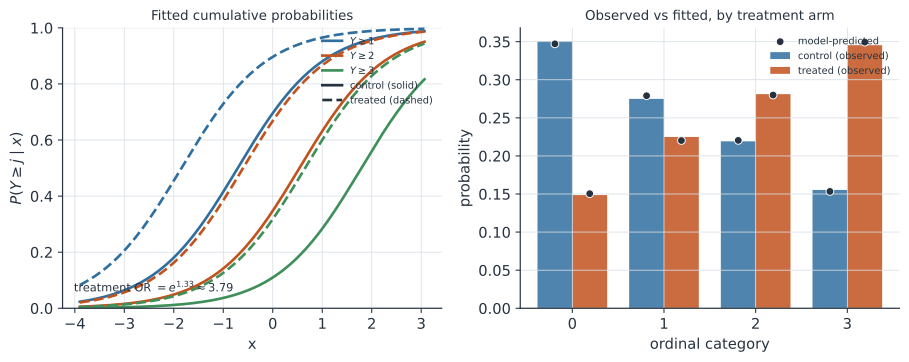
print("treatment odds ratio:", round(float(np.exp(b[1])), 3))   # recovers ~exp(1.3)

slopes (x, treat): [1.17  1.331]
treatment odds ratio: 3.787

The fit from the code above. Left: the model’s fitted cumulative probabilities for control (solid) and treated (dashed); treatment shifts every curve by the same single odds ratio printed above, . Right: the model reproduces the data — observed category proportions (bars) versus model-predicted (dots), split by treatment arm, with treatment moving mass toward the highest category. — Figure 3. The fit from the code above. Left: the model’s fitted cumulative probabilities $P(Y \ge j \mid x)$ for control (solid) and treated (dashed); treatment shifts every curve by the same single odds ratio printed above, $e^{1.33} \approx 3.79$ . Right: the model reproduces the data — observed category proportions (bars) versus model-predicted (dots), split by treatment arm, with treatment moving mass toward the highest category.

Julia#

Julia

# Cumulative-link (proportional odds) model via GLM's ordinal support
using MixedModels, DataFrames, CategoricalArrays   # or the Ordinal.jl ecosystem
# Illustrative: fit an ordered outcome with a logit cumulative link.
# Packages: `Econometrics.jl` and `GLM.jl` provide proportional-odds fits;
# the shared-slope structure mirrors the R/Python calls above.

Why it matters#

Ordinal outcomes are everywhere in health research — symptom severity, functional and disability scales, tumor grade, Likert-scale patient-reported outcomes, and the ordinal clinical-status scales that became standard endpoints in COVID-19 trials. The proportional odds model lets you analyze them without discarding the ordering and without pretending the categories are equally spaced numbers, and it delivers a single odds ratio that clinicians and regulators can read.

Seeing it as one point on a continuum — binary logistic regression at one end, the Cox model and survival analysis at the other, all linear models for the log-odds or log-hazard of crossing a threshold — is what lets you choose the right member of the family for a given outcome, and defend the choice. Frank Harrell’s central message, argued across his Regression Modeling Strategies and Statistical Thinking blog, is that the ordinal model’s assumptions are milder than the alternatives’, its power is higher, and a violation of proportional odds is a reason to assess impact — not a reason to dichotomize.

Logistic Regression — the two-category special case
Cox Proportional Hazards Regression — the same idea with a complementary-log-log link
Survival Analysis — ordered event times with censoring
Generalized Linear Models
Maximum Likelihood
Contrasts and Average Marginal Effects
Monotonic Transformations — why invariance to recoding $Y$ matters
Quantitative Methods