Queueing Theory and ICU Colonization

An intensive care unit is a queue. Patients (the customers) arrive, occupy a bed (the server) for a while, and leave; when every bed is full a new arrival is diverted elsewhere. Layered on top of that flow is an epidemiological process: while they share the unit, patients can pass a colonizing organism — MRSA, VRE, or a carbapenem-resistant Enterobacterales — to one another via the hands of staff and shared surfaces. Queueing theory describes who is in the beds and how fast they turn over; a small Markov chain on top describes how many of them are colonized, and together they tell you the endemic prevalence and how much each infection-prevention (IP) practice actually buys.

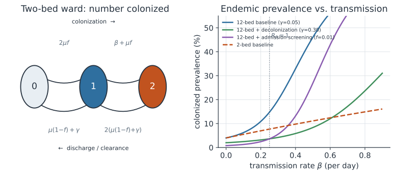
The ward as a queue#

Strip out colonization for a moment and just watch the beds. Admissions arrive as a Poisson process at rate $\lambda$, each patient stays for an exponentially distributed length of stay with mean $1/\mu$, and there are $c$ beds and no waiting room — a full ICU turns patients away rather than queueing them. This is the M/M/$c$/$c$ (Erlang loss) system, and the chance an arrival finds all $c$ beds full is the Erlang-B formula $$B(c, a) = \frac{a^c/c!}{\sum_{k=0}^{c} a^k/k!}, \qquad a = \lambda/\mu,$$ with $a$ the offered load in Erlangs. For a busy unit the occupancy sits close to $c$, so from here on we take the ward to be full, and read $\mu$ as the per-bed turnover rate: every bed empties and refills at rate $\mu$, mean stay $1/\mu$.

A two-bed ward as a birth-death chain#

Now add the bug. Let the state $X$ be the number of colonized patients among the occupied beds; in a two-bed bay $X \in \{0, 1, 2\}$. Three rates move it.

• Cross-transmission. A colonized patient colonizes a susceptible ward-mate at rate $\beta$ (per susceptible), the parameter that hand hygiene and contact precautions act on. With $X$ colonized and $N-X$ susceptible in an $N$-bed ward, the total colonization rate from transmission is $\beta\, X (N-X)/(N-1)$, scaled so a single carrier among otherwise-susceptible beds transmits at rate $\beta$.
• Importation. A susceptible bed turns over at rate $\mu$, and the incoming patient is already colonized with probability $f$ (the admission prevalence), adding susceptible-to-colonized flow $\mu f (N-X)$.
• Loss. A colonized patient leaves the colonized pool either by being discharged and replaced by a susceptible admission, at rate $\mu(1-f)$, or by clearing carriage (spontaneously or through decolonization) at rate $\gamma$. Per colonized patient the down-rate is $\mu(1-f) + \gamma$.

For $N = 2$ this is a birth-death chain with up-rates $b_0 = 2\mu f$ (both beds can import) and $b_1 = \beta + \mu f$ (transmission to the one susceptible, plus its import risk), and down-rates $d_1 = \mu(1-f)+\gamma$ and $d_2 = 2\big(\mu(1-f)+\gamma\big)$ (Figure 1, left). A birth-death chain satisfies detailed balance, so the stationary distribution follows by multiplying the ratios up the ladder: $$\pi_1 = \pi_0\,\frac{b_0}{d_1}, \qquad \pi_2 = \pi_1\,\frac{b_1}{d_2}, \qquad \pi_0 + \pi_1 + \pi_2 = 1 .$$

The ward reproduction number#

One summary decides whether transmission can sustain itself inside the unit. A newly colonized patient transmits at rate $\beta$ and stays colonized-and-present for a mean time $1/(\mu + \gamma)$ before being discharged or clearing, so it generates $$R_A = \frac{\beta}{\mu + \gamma} \tag{1}$$ secondary colonizations — the ward reproduction number, the hospital analog of $R_0$. When $R_A > 1$, colonization is self-sustaining: it persists through in-ward spread even if no one is ever admitted already carrying ($f = 0$). When $R_A < 1$, in-ward chains fade out on their own and prevalence is importation-driven — kept alight only by colonized admissions, so controlling who comes in matters more than controlling spread once they are there. Notice importation $f$ does not appear in (1): it seeds outbreaks but does not change the threshold.

Scaling up to a full unit#

Nothing above was special to two beds. For an $N$-bed unit the same three mechanisms give a birth-death chain on $X \in \{0, \dots, N\}$ with $$b_X = \underbrace{\beta\,\frac{X(N-X)}{N-1}}_{\text{transmission}} + \underbrace{\mu f\,(N-X)}_{\text{importation}}, \qquad d_X = \big(\mu(1-f) + \gamma\big)\,X ,$$ and the stationary prevalence $\mathbb{E}[X]/N$ follows from the same detailed-balance product. This is exactly an SIS epidemic running in a demographically open population — the ward — with importation playing the role of an external reservoir.

Ward size matters more than the mean-field intuition suggests. Because transmission is frequency-dependent, $R_A$ in (1) does not depend on $N$, yet the endemic prevalence does: in a tiny bay, chance fade-out repeatedly extinguishes transmission, whereas a large unit sustains it. The same per-encounter transmissibility that barely simmers in a two-bed bay can hold a twelve-bed unit at high prevalence — the hospital version of a critical community size (Figure 1, right).

Infection-prevention levers#

Each IP practice is a specific parameter change, and (1) and the stationary distribution price them out.

Two practices can hit the same threshold by different routes: halving $\beta$ and raising $\gamma$ enough both drive $R_A$ to $1$, but decolonization also shortens carriage, so it tends to lower prevalence a little more per unit of $R_A$. When $R_A$ is already below $1$, the residual prevalence is all importation, and screening (lowering $f$) does the heavy lifting that hand hygiene no longer can.

A worked example#

Take a two-bed bay with turnover $\mu = 0.2\,\text{day}^{-1}$ (mean stay $5$ days), spontaneous clearance $\gamma = 0.05\,\text{day}^{-1}$, admission prevalence $f = 0.05$, and transmission $\beta = 0.5\,\text{day}^{-1}$, so $R_A = 0.5/0.25 = 2$. The per-colonized loss rate is $\mu(1-f)+\gamma = 0.2(0.95) + 0.05 = 0.24$, giving up-rates $b_0 = 2(0.2)(0.05) = 0.02$ and $b_1 = 0.5 + 0.01 = 0.51$, and down-rates $d_1 = 0.24$, $d_2 = 0.48$. Detailed balance gives $\pi_1/\pi_0 = 0.02/0.24 = 0.0833$ and $\pi_2/\pi_1 = 0.51/0.48 = 1.0625$, which normalize to $\pi \approx (0.853,\ 0.071,\ 0.076)$. The colonized prevalence is $\mathbb{E}[X]/2 = (0.071 + 2\cdot 0.076)/2 \approx 11\%$. In a twelve-bed unit the same parameters give roughly $46\%$ colonized — four times higher — precisely the ward-size effect above. Halving $\beta$ with hand hygiene, or raising $\gamma$ with decolonization, drops both figures sharply, as the code below tabulates.

In code#

We build the generator, solve for the stationary prevalence exactly by detailed balance, and cross-check it with a Gillespie simulation.

R#

stationary <- function(N, beta, mu, gamma, f) {
  X <- 0:N; Sus <- N - X
  b <- ifelse(N > 1, beta * X * Sus / (N - 1), 0) + mu * f * Sus  # up
  d <- (mu * (1 - f) + gamma) * X                                 # down
  logpi <- c(0, cumsum(log(b[1:N]) - log(d[2:(N + 1)])))          # detailed balance
  pi <- exp(logpi - max(logpi)); pi <- pi / sum(pi)
  list(pi = pi, prevalence = sum(X * pi) / N)
}

mu <- 0.2; f <- 0.05
for (s in list(c(0.50, 0.05), c(0.25, 0.05), c(0.50, 0.30), c(0.25, 0.30))) {
  p2  <- stationary(2,  s[1], mu, s[2], f)$prevalence
  p12 <- stationary(12, s[1], mu, s[2], f)$prevalence
  cat(sprintf("R_A=%.2f  2-bed=%.1f%%  12-bed=%.1f%%\n",
              s[1] / (mu + s[2]), 100 * p2, 100 * p12))
}

Python#

import numpy as np

def stationary(N, beta, mu, gamma, f):
    """Birth-death CTMC for the number colonized in a full N-bed ward."""
    b = np.zeros(N + 1)                        # colonization (up) rates
    d = np.zeros(N + 1)                        # loss (down) rates
    for X in range(N + 1):
        Sus = N - X
        transmission = beta * X * Sus / (N - 1) if N > 1 else 0.0
        b[X] = transmission + mu * f * Sus     # cross-transmission + importation
        d[X] = (mu * (1 - f) + gamma) * X      # discharge-to-susceptible + clearance
    pi = np.ones(N + 1)
    for X in range(1, N + 1):
        pi[X] = pi[X - 1] * b[X - 1] / d[X]    # detailed balance up the ladder
    pi /= pi.sum()
    return pi, (np.arange(N + 1) * pi).sum() / N

mu, f = 0.2, 0.05
print("practice          R_A   2-bed   12-bed")
for name, beta, gamma in [("baseline",       0.50, 0.05),
                          ("hand hygiene",   0.25, 0.05),
                          ("decolonization", 0.50, 0.30),
                          ("both",           0.25, 0.30)]:
    _, p2  = stationary(2,  beta, mu, gamma, f)
    _, p12 = stationary(12, beta, mu, gamma, f)
    print(f"{name:15s} {beta / (mu + gamma):5.2f}  {p2:5.1%}  {p12:5.1%}")

practice          R_A   2-bed   12-bed
baseline         2.00  11.1%  46.0%
hand hygiene     1.00   7.7%  14.8%
decolonization   1.00   3.9%   8.3%
both             0.50   3.0%   3.6%

A stochastic simulation of the same generator confirms the exact prevalence.

def gillespie_prevalence(N, beta, mu, gamma, f, T, seed):
    rng = np.random.default_rng(seed)
    X, t, colonized_bed_days = 0, 0.0, 0.0
    while t < T:
        Sus = N - X
        up = beta * X * Sus / (N - 1) + mu * f * Sus
        down = (mu * (1 - f) + gamma) * X
        rate = up + down
        dt = rng.exponential(1 / rate)
        colonized_bed_days += X * dt           # time-integral of colonized count
        t += dt
        X += 1 if rng.random() < up / rate else -1
    return colonized_bed_days / (t * N)         # long-run colonized prevalence

sim = gillespie_prevalence(12, 0.50, mu, 0.05, f, T=100_000, seed=1)
_, exact = stationary(12, 0.50, mu, 0.05, f)
print(round(sim, 2), round(exact, 2))           # simulated vs exact prevalence

0.46 0.46

Julia#

function stationary(N, beta, mu, gamma, f)
    X = 0:N; Sus = N .- X
    b = (N > 1 ? beta .* X .* Sus ./ (N - 1) : zeros(N + 1)) .+ mu * f .* Sus
    d = (mu * (1 - f) + gamma) .* X
    logpi = cumsum(vcat(0.0, log.(b[1:N]) .- log.(d[2:N+1])))
    pi = exp.(logpi .- maximum(logpi)); pi ./= sum(pi)
    (pi, sum(X .* pi) / N)
end

mu, f = 0.2, 0.05
for (beta, gamma) in [(0.50, 0.05), (0.25, 0.05), (0.50, 0.30), (0.25, 0.30)]
    _, p2  = stationary(2,  beta, mu, gamma, f)
    _, p12 = stationary(12, beta, mu, gamma, f)
    println("R_A=", round(beta / (mu + gamma); digits = 2),
            "  2-bed=", round(100p2; digits = 1),
            "%  12-bed=", round(100p12; digits = 1), "%")
end

Why it matters#

Colonization is the reservoir from which hospital infections and resistant-organism outbreaks erupt, and control budgets are finite, so the question is always which lever to pull. Casting the ward as a queue with a colonization chain on top separates the two forces that keep a bug endemic — in-ward transmission ($R_A$) and importation ($f$) — and shows that they call for different responses: hand hygiene and cohorting when $R_A > 1$, admission screening when the unit is running on imports. It also explains why the same organism can smoulder in a small step-down unit yet blaze in a large ICU, why understaffing (which effectively raises $\beta$) shows up as outbreaks, and how to compare a bundle of interventions before spending on any of them.

Related#

• Markov Chains
• Stochastic Epidemics and the Gillespie Algorithm
• SEIR and Compartmental Extensions
• The Next-Generation Matrix and R₀
• Poisson Distribution
• Population Dynamics of Resistance
• Quantitative Methods