Response Surface Methodology

Response Surface Methodology (RSM) is a sequential strategy for optimizing a process or output over continuous factors — think maximizing yield or minimizing defects by tuning temperature and pressure. You first move quickly toward the optimum with a simple model, then map the curvature near it with a richer one.

Figure 1. Left: the two-phase strategy — far from the optimum the fitted plane’s gradient gives the direction of steepest ascent, so experimental steps climb toward the peak before a second-order model maps the curvature there. Right: a central composite design builds the three levels a quadratic needs from three pieces — the

2^k

factorial corners,

2k

axial (star) points at radius

\alpha

, and replicated center points.

The two-phase strategy#

Phase 1: first-order model and steepest ascent#

Far from the optimum, the surface is locally well approximated by a plane:

$y = \beta_0 + \sum_{i=1}^{k} \beta_i x_i + \varepsilon.$

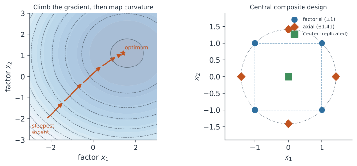
Fit it with a two-level factorial plus center points. The gradient $(\beta_1, \dots, \beta_k)$ points in the direction of steepest ascent; take experimental steps along it until the response stops improving, signaling you are near a peak (where first-order terms flatten and curvature dominates) (Figure 1).

Phase 2: second-order model and curvature#

Near the optimum, add quadratic and cross-product terms:

$y = \beta_0 + \sum_{i} \beta_i x_i + \sum_{i} \beta_{ii} x_i^2 + \sum_{i<j} \beta_{ij} x_i x_j + \varepsilon.$

This quadratic can bend, so it can represent a maximum, minimum, or saddle.

Central composite designs (CCD)#

Fitting the second-order model requires at least three levels per factor. A central composite design builds this economically from three pieces:

Factorial points — the $2^k$ (or fractional) corners, $x_i = \pm 1$ .
Axial (star) points — $2k$ points at $(\pm\alpha, 0, \dots, 0)$ , etc., extending each axis beyond the cube. Choosing $\alpha = (2^k)^{1/4}$ gives a rotatable design (equal prediction variance at equal distance from the center).
Center points — several replicates at the origin, giving a pure-error estimate and information on curvature.

Canonical / stationary-point analysis#

Write the fitted second-order model in matrix form:

$\hat y = \beta_0 + x^\top b + x^\top B x,$

where $b$ is the vector of linear coefficients and $B$ is the symmetric matrix with $\beta_{ii}$ on the diagonal and $\beta_{ij}/2$ off-diagonal. Setting the gradient to zero, $\,b + 2Bx = 0$ , gives the stationary point:

$x_s = -\tfrac{1}{2} B^{-1} b.$

The eigenvalues of $B$ classify it: all negative → maximum, all positive → minimum, mixed signs → saddle point (a ridge to explore further).

Worked example#

Fit a one-factor quadratic $\hat y = \beta_0 + \beta_1 x + \beta_{11} x^2$ . With scalar $b = \beta_1$ and $B = \beta_{11}$ , the stationary point is

$x_s = -\frac{\beta_1}{2\beta_{11}}.$

Suppose $\hat y = 80 + 6x - 3x^2$ . Then $x_s = -6 / (2 \cdot -3) = 1.0$ , and since $\beta_{11} = -3 < 0$ it is a maximum, with predicted optimum $\hat y = 80 + 6(1) - 3(1)^2 = 83$ . In two factors the same formula $x_s = -\tfrac12 B^{-1}b$ locates the peak of the fitted surface.

In code#

R#

library(rsm)
set.seed(1)
# Central composite design in 2 coded factors
d <- ccd(2, n0 = c(3, 3), alpha = "rotatable", randomize = FALSE)
# Simulate a quadratic response with a maximum
d$y <- 80 + 6 * d$x1 + 4 * d$x2 - 3 * d$x1^2 - 2 * d$x2^2 -
       d$x1 * d$x2 + rnorm(nrow(d), 0, 0.5)

fit <- rsm(y ~ SO(x1, x2), data = d)   # SO = second order
summary(fit)                            # includes stationary point + eigenvalues

Python#

Python

import numpy as np
import pandas as pd
import statsmodels.formula.api as smf
from pyDOE3 import ccdesign

np.random.seed(1)
pts = ccdesign(2, center=(3, 3), alpha="r", face="ccc")  # rotatable CCD
d = pd.DataFrame(pts, columns=["x1", "x2"])
d["y"] = (80 + 6*d.x1 + 4*d.x2 - 3*d.x1**2 - 2*d.x2**2
          - d.x1*d.x2 + np.random.normal(0, 0.5, len(d)))

fit = smf.ols("y ~ x1 + x2 + I(x1**2) + I(x2**2) + x1:x2", data=d).fit()
c = fit.params
b = np.array([c["x1"], c["x2"]])
B = np.array([[c["I(x1 ** 2)"], c["x1:x2"] / 2],
              [c["x1:x2"] / 2,  c["I(x2 ** 2)"]]])
x_s = -0.5 * np.linalg.solve(B, b)
print(x_s)                 # stationary point ~ (0.9, 0.8)
print(np.linalg.eigvals(B))  # both negative -> maximum

Julia#

Julia

using LinearAlgebra, Random
Random.seed!(1)

# Manual CCD in 2 factors: factorial corners, axial points, center reps
α = 2.0^(1/4)                         # rotatable
factorial_pts = [(-1,-1), (1,-1), (-1,1), (1,1)]
axial_pts     = [(-α,0), (α,0), (0,-α), (0,α)]
center_pts    = fill((0.0, 0.0), 3)
pts = vcat(collect.(factorial_pts), collect.(axial_pts), collect.(center_pts))
X1 = [p[1] for p in pts]; X2 = [p[2] for p in pts]

y = 80 .+ 6 .*X1 .+ 4 .*X2 .- 3 .*X1.^2 .- 2 .*X2.^2 .- X1.*X2 .+ 0.5 .*randn(length(pts))

# Design matrix: 1, x1, x2, x1^2, x2^2, x1*x2 ; least squares
X = hcat(ones(length(pts)), X1, X2, X1.^2, X2.^2, X1.*X2)
β = X \ y
b = [β[2], β[3]]
B = [β[4]      β[6]/2;
     β[6]/2    β[5]]
x_s = -0.5 * (B \ b)      # stationary point
eigvals(B)                 # both negative -> maximum

Why it matters for statistics#

RSM turns optimization into a sequence of small, informative experiments rather than a blind search. By pairing efficient designs (factorials, then CCDs) with regression models and calculus (gradients for ascent, the stationary-point formula for the peak), it finds and characterizes optima with minimal runs. It is central to process improvement in chemistry, manufacturing, and formulation science, and it connects experimental design directly to continuous optimization.