Splines and Penalized Regression

Straight lines rarely describe biology. Risk of death is not linear in age, an exposure–response curve bends and saturates, and a seasonal signal rises and falls — yet we still want the flexibility of a smooth curve without hand-picking a transformation or a polynomial degree. Splines give us that: they build a flexible curve out of simple polynomial pieces joined smoothly at a set of knots, turning “fit a smooth function of $x$” into an ordinary linear regression on a handful of constructed columns.

The idea: piecewise polynomials joined smoothly#

Fitting one global high-degree polynomial to bendy data is a bad idea — it oscillates wildly and lets a point on the left dictate the fit on the right (overfitting). A spline instead divides the range of $x$ at a set of knots $t_1 < t_2 < \cdots < t_K$ and fits a low-degree polynomial (usually cubic) within each interval, subject to smoothness constraints where the pieces meet.

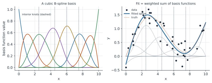
For a cubic spline the constraints are that at every interior knot the neighboring cubics agree in value, first derivative, and second derivative. Those constraints are exactly enough to make the joins invisible: the curve and its slope and curvature are continuous, so the eye sees one smooth function rather than a chain of segments (Figure 1). Each additional knot buys one more degree of freedom — one more wiggle the curve is allowed.

From constraints to a basis#

The practical trick is that the set of all cubic splines with a fixed set of knots is a finite-dimensional vector space: every such spline is a linear combination of a fixed set of basis functions $b_1(x),\dots,b_m(x)$, $$f(x) = \sum_{j=1}^{m} \beta_j\, b_j(x). \tag{1}$$ Once you have the basis, fitting a spline is linear regression — you build the design-matrix columns $b_j(x_i)$ and estimate $\beta$ by least squares or, for non-Gaussian outcomes, as a GLM. The whole apparatus of standard errors, confidence bands, and likelihood-ratio tests comes along for free.

Different bases span the same space of curves but differ in numerical behavior:

• The truncated power basis $\{1, x, x^2, x^3, (x-t_1)_+^3, \dots, (x-t_K)_+^3\}$, where $(u)_+ = \max(u,0)$, is the textbook construction — transparent but badly conditioned.
• The B-spline basis (Figure 1, left) spans the identical space but each basis function is a localized bump, nonzero over only a few adjacent knot spans. That locality makes the design matrix banded and the fit numerically stable; it is the standard construction, developed in Carl de Boor’s A Practical Guide to Splines (de Boor 1978).

Restricted cubic (natural) splines#

An unconstrained cubic spline has a weakness at the edges: beyond the outermost knots, where data are sparse, the cubic pieces are free to curve dramatically, so predictions and confidence intervals blow up in the tails.

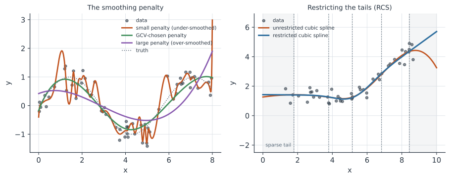
The restricted cubic spline (RCS), also called a natural spline, fixes this by adding two boundary constraints: the function is forced to be linear beyond the two outer knots. This is the spline that Frank Harrell recommends as a default in Regression Modeling Strategies (Harrell 2015; free course notes at hbiostat.org/rms), building on Stone and Koo (1985) and Durrleman and Simon (1989). Linear tails cost two degrees of freedom, so an RCS with $K$ knots uses only $K-1$ parameters (including the intercept), and the sparse, high-leverage tail regions no longer drive the fit (Figure 2, right).

Harrell’s rcs() uses a rescaled truncated-power construction so that the first basis column is $x$ itself, which makes the linear-tail behavior explicit and lets a single test isolate departure from linearity.

Penalized (smoothing) splines#

Choosing the number of knots is really a choice about smoothness, and it is discrete and fiddly. The alternative that dominates modern practice is to use many knots — enough to be flexible — but to add a roughness penalty that discourages wiggliness, then tune one continuous smoothing parameter.

A smoothing spline minimizes a penalized sum of squares, $$\sum_{i=1}^{n}\bigl(y_i - f(x_i)\bigr)^2 \;+\; \lambda \int f''(x)^2\,dx, \tag{2}$$ where $\int f''(x)^2\,dx$ measures total curvature and $\lambda \ge 0$ controls the trade-off. Remarkably, the exact minimizer of (2) over all twice-differentiable functions is a natural cubic spline with a knot at every distinct $x_i$ — a classical result at the heart of Green and Silverman (1994). The penalty, not the knot count, now does the regularizing:

• $\lambda \to 0$: no penalty, the curve interpolates the noise (under-smoothed, high variance);
• $\lambda \to \infty$: the penalty forces $f''=0$, collapsing to the ordinary least-squares straight line (over-smoothed, high bias);
• intermediate $\lambda$: the bias–variance trade-off is balanced (Figure 2, left).

In matrix form the penalty is a quadratic $\lambda\,\beta^\top S \beta$ for a fixed penalty matrix $S$, so the estimator is penalized (ridge-like) least squares, $$\hat\beta = \bigl(B^\top B + \lambda S\bigr)^{-1} B^\top y,$$ with $B$ the basis design matrix. Because the fit is a linear smoother $\hat y = A(\lambda)\,y$, its complexity is summarized by the effective degrees of freedom $\mathrm{edf} = \operatorname{tr} A(\lambda)$ — a continuous analogue of “number of parameters” that shrinks from the basis dimension toward $2$ (a line) as $\lambda$ grows.

P-splines#

A computationally convenient version replaces the integral penalty with a discrete one. Eilers and Marx (1996) proposed P-splines: a B-spline basis on evenly spaced knots plus a penalty on differences of adjacent coefficients, $\lambda\sum_j (\Delta^2 \beta_j)^2$. Penalizing second differences keeps neighboring coefficients close, which mimics the curvature penalty of (2) while being trivial to compute and easy to extend (to different difference orders, to varying penalties, to non-Gaussian responses). They are the "ps" smoother in Simon Wood’s mgcv.

Thin plate (regression) splines#

In one dimension “roughness” is curvature. In two or more dimensions — think a smooth surface over spatial coordinates, or a smooth interaction $f(x_1, x_2)$ — the natural generalization is the thin plate spline, which penalizes the bending energy of a thin metal sheet, $$\iint \left[ \left(\tfrac{\partial^2 f}{\partial x_1^2}\right)^2 + 2\left(\tfrac{\partial^2 f}{\partial x_1 \partial x_2}\right)^2 + \left(\tfrac{\partial^2 f}{\partial x_2^2}\right)^2 \right] dx_1\,dx_2.$$ Thin plate splines are knot-free and isotropic (rotationally invariant): you never choose knots, and the smoother treats all directions the same, which makes them a principled default for smoothing over space or over several covariates at once.

Their catch is cost — a classical thin plate spline uses one basis function per data point, so it does not scale. Simon Wood (2003) solved this with thin plate regression splines: an eigen-decomposition produces an optimal low-rank approximation that keeps almost all of the smoothing behavior of the full thin plate spline at a fraction of the cost. This "tp" construction is the default smoother in mgcv and is why you can write s(x) in a model formula and get a well-behaved penalized smooth with no knot bookkeeping.

Choosing the smoothness automatically#

The one number left to choose is $\lambda$ (or, equivalently, the edf). Two principled, data-driven criteria dominate, both central to Wood’s mgcv:

• Generalized cross-validation (GCV) approximates leave-one-out prediction error as a closed-form function of $\lambda$, avoiding an explicit CV loop.
• Restricted maximum likelihood (REML) treats the penalty as a Gaussian prior — a spline is formally a mixed model with the wiggly component as a random effect — and estimates $\lambda$ as a variance component.

Wood’s stable REML/GCV machinery (Wood 2011) is what makes GAM fitting turnkey; REML is generally preferred because it is less prone to occasional severe under-smoothing than GCV. This mixed-model view is the bridge from splines to Gaussian processes and hierarchical models: a penalized spline is a random-effects model, and the smoothing parameter is a ratio of variances.

Worked example: how many knots is that, really?#

Suppose we model log-hazard as a smooth function of age with a restricted cubic spline at $K=4$ knots. The RCS spends $K-1 = 3$ regression degrees of freedom: one for the linear term and $K-2 = 2$ for the nonlinear basis columns. So a test of “is age’s effect nonlinear?” is a 2-degree-of-freedom test on those two columns — if it is not significant, you drop them and report a simple linear age effect.

Now suppose instead we fit a penalized smooth s(age) in mgcv with a basis dimension of $10$ and REML picks a smoothing parameter giving $\mathrm{edf} = 3.8$. That single curve is “worth” about $3.8$ parameters — more flexible than the 4-knot RCS, but the penalty, not a knot count, decided how much. The two philosophies meet in the middle: fix a small basis and test (Harrell’s RCS style) or oversize the basis and penalize (Wood’s GAM style).

In code#

R#

## --- Simon Wood's mgcv: penalized smooths, smoothness by REML ---
library(mgcv)
set.seed(1)
d <- data.frame(x = sort(runif(200, 0, 10)))
d$y <- sin(0.7 * d$x) + 0.2 * d$x + rnorm(200, 0, 0.3)

m_tp <- gam(y ~ s(x, bs = "tp"), data = d, method = "REML")  # thin plate (default)
m_ps <- gam(y ~ s(x, bs = "ps"), data = d, method = "REML")  # P-spline
summary(m_tp)          # edf = effective degrees of freedom of the smooth
plot(m_tp, shade = TRUE)

## --- Frank Harrell's rms: restricted cubic splines, fixed knots ---
library(rms)
dd <- datadist(d); options(datadist = "dd")
f <- ols(y ~ rcs(x, 4), data = d)   # RCS, 4 knots at default quantiles
anova(f)               # includes an explicit test of NONLINEARITY
Predict(f, x)          # fitted curve with confidence band

Python#

import numpy as np
from scipy.interpolate import make_smoothing_spline

rng = np.random.default_rng(0)
x = np.sort(rng.uniform(0, 10, 120))
y = np.sin(0.7 * x) + 0.2 * x + rng.normal(0, 0.3, x.size)

# Penalized smoothing spline; lambda chosen automatically by GCV
spl = make_smoothing_spline(x, y)
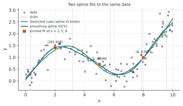
print("smoothing-spline fit at x=2,5,8:", np.round(spl([2.0, 5.0, 8.0]), 3))

# Harrell-style restricted cubic spline basis (linear beyond outer knots)
def rcs(x, knots):
    x = np.asarray(x, float); k = np.asarray(knots, float); K = len(k)
    tk1, tkK = k[-2], k[-1]; d = tkK - tk1
    cube = lambda u: np.where(u > 0, u, 0.0) ** 3
    cols = [x]
    for j in range(K - 2):
        cols.append((cube(x - k[j])
                     - cube(x - tk1) * (tkK - k[j]) / d
                     + cube(x - tkK) * (tk1 - k[j]) / d) / d ** 2)
    return np.column_stack(cols)

knots = np.quantile(x, [0.05, 0.275, 0.50, 0.725, 0.95])   # 5 knots
B = np.column_stack([np.ones(x.size), rcs(x, knots)])
beta, *_ = np.linalg.lstsq(B, y, rcond=None)
print("rcs coefficients (intercept, linear, nonlinear...):", np.round(beta, 3))

smoothing-spline fit at x=2,5,8: [1.408 0.696 0.987]
rcs coefficients (intercept, linear, nonlinear...): [ 0.14   0.661 -0.098  0.31  -0.285]

Julia#

# Penalized/basis splines via BSplineKit.jl (illustrative)
using BSplineKit, Random
Random.seed!(1)
x = sort(rand(120) .* 10)
y = sin.(0.7 .* x) .+ 0.2 .* x .+ 0.3 .* randn(120)

# Cubic B-spline basis on a set of interior breakpoints, then least-squares fit
breaks = range(0, 10; length = 8)
B = BSplineBasis(BSplineOrder(4), collect(breaks))   # order 4 = cubic
S = SplineInterpolation(B, x, y)                     # or SmoothingSpline for a penalty
S.(0:2:10)

Why it matters#

Splines are the workhorse for nonlinearity across quantitative epidemiology: exposure–response curves that bend, mortality that accelerates with age, seasonal and long-term time trends in surveillance series, and smooth spatial surfaces for disease mapping. They are the smooth terms $s(\cdot)$ inside generalized additive models, the flexible baseline in flexible-parametric survival models, and the smoothers behind estimates of the time-varying reproduction number.

The two traditions here are complementary, not rival. Frank Harrell’s restricted cubic splines emphasize pre-specifying a small, interpretable number of knots and testing nonlinearity honestly within a regression-modeling workflow. Simon Wood’s penalized thin plate and P-splines emphasize oversizing the basis and letting REML choose the smoothness, which scales to surfaces and to automatic model building. Knowing both lets you pick nonlinearity that is flexible and accountable — and to read a spline term in someone else’s model without mistaking flexibility for overfitting.

Related#

• Linear Regression
• Generalized Linear Models
• Overfitting, Regularization, and Cross-Validation
• Gaussian Processes — the mixed-model / kernel cousin of penalized splines
• Hierarchical (Multilevel) Models — a spline is a random-effects model
• Covariance Functions and the Matérn Family
• Bayesian Spatial Models with INLA — SPDE smooths as splines/GPs
• Quantitative Methods