Numerical Methods for Dynamical Systems
Most dynamical models in biology — SIR and SEIR epidemics, predator–prey systems, pharmacokinetics, gene-regulatory circuits — are written as differential equations that have no closed-form solution. To see how the model behaves you must integrate it numerically: step the system forward in small time increments. The catch is that the numerical answer is only an approximation, and a careless choice of method or step size can produce a curve that looks plausible but is quantitatively — or even qualitatively — wrong.
This page is about getting trustworthy trajectories out of your models.
Stepping Forward in Time#
An ODE tells you the rate of change, , and you know where you start. A numerical integrator turns that local slope into a full trajectory by taking small steps of size .
The simplest is Euler’s method: follow the current slope for one step.
It is easy to understand and easy to code — and rarely what you should actually use, because its error is large and it can be unstable.
A far better default is fourth-order Runge–Kutta (RK4), which samples the slope four times within each step and combines them. It is only a little more code but dramatically more accurate for the same step size.
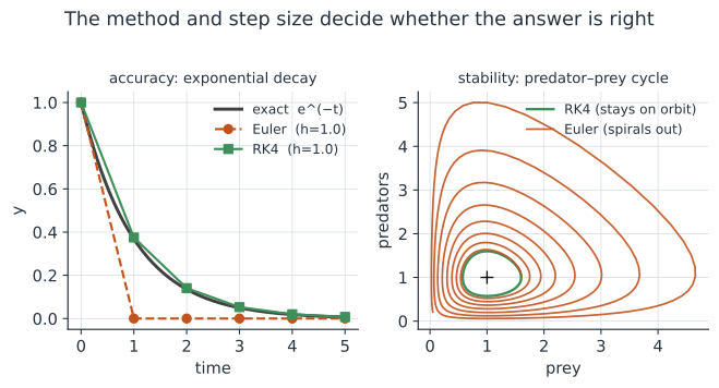
The figure shows both failure modes. On the left, Euler with a big step badly undershoots simple exponential decay while RK4 stays on the exact curve. On the right — the more insidious case — a predator–prey system that should cycle forever on a closed loop is integrated by Euler into an outward spiral, silently inventing population growth that is nowhere in the equations. RK4 stays on the orbit.
Step Size and Accuracy#
Euler’s error per step shrinks in proportion to (it is a first-order method), so halving the step roughly halves the error. RK4’s error shrinks with , so halving the step cuts the error by about sixteen-fold — which is why RK4 reaches a given accuracy with far larger steps.
You can watch Euler’s first-order convergence directly:
import numpy as np

def euler_decay(k, y0, h, T):
    """Integrate y' = -k y from 0 to T with step h."""
    y, n = y0, int(round(T / h))
    for _ in range(n):
        y += h * (-k * y)
    return y

T, exact = 5.0, np.exp(-1.0 * 5.0)      # true value of y(5) for k=1, y0=1
for h in [1.0, 0.5, 0.1, 0.01]:
    approx = euler_decay(1.0, 1.0, h, T)
    print(f"h={h:>5}:  euler={approx:.5f}   error={abs(approx - exact):.5f}")
h=  1.0:  euler=0.00000   error=0.00674
h=  0.5:  euler=0.00098   error=0.00576
h=  0.1:  euler=0.00515   error=0.00158
h= 0.01:  euler=0.00657   error=0.00017
Each 10-fold smaller step gives roughly a 10-fold smaller error — the signature of a first-order method, and a reminder that Euler buys accuracy only by taking many tiny steps.
Stiffness: When Small Steps Are Forced#
A system is stiff when it contains processes on very different timescales — a fast reaction alongside a slow one, which is common in biochemical and multi-scale epidemic models. Explicit methods like Euler and RK4 are then forced to take absurdly small steps for stability, not accuracy: exceed a critical step size and the solution explodes into oscillations even though the true dynamics are smooth.
The fix is an implicit or adaptive solver (ode23s, LSODA, Rodas, backward-differentiation methods) that detects stiffness and adjusts.
The practical signal: if your integration blows up or crawls no matter how you tune it, suspect stiffness and switch to a stiff solver.
Don’t Hand-Roll It — Use a Solver#
Euler and RK4 above are for understanding. For real work, call a mature adaptive solver: it chooses the step size for you, controls the error to a tolerance you set, and handles stiffness.
# R: deSolve -- the standard ODE integrator
library(deSolve)
sir <- function(t, y, p) {
  with(as.list(c(y, p)), {
    dS <- -beta * S * I
    dI <-  beta * S * I - gamma * I
    dR <-  gamma * I
    list(c(dS, dI, dR))
  })
}
out <- ode(y = c(S = 0.99, I = 0.01, R = 0),
           times = seq(0, 60, 0.1),
           func = sir, parms = c(beta = 0.4, gamma = 0.1))
# Julia: DifferentialEquations.jl -- picks a good method automatically
using DifferentialEquations
function sir!(du, u, p, t)
    S, I, R = u; β, γ = p
    du[1] = -β*S*I
    du[2] =  β*S*I - γ*I
    du[3] =  γ*I
end
prob = ODEProblem(sir!, [0.99, 0.01, 0.0], (0.0, 60.0), (0.4, 0.1))
sol  = solve(prob)                 # adaptive step, stiffness-aware
# Python: SciPy's solve_ivp with an adaptive method
from scipy.integrate import solve_ivp

def sir(t, y, beta, gamma):
    S, I, R = y
    return [-beta*S*I, beta*S*I - gamma*I, gamma*I]

sol = solve_ivp(sir, (0, 60), [0.99, 0.01, 0.0],
                args=(0.4, 0.1), method="LSODA",   # switches if stiff
                rtol=1e-6, dense_output=True)
Set the tolerances (rtol/atol) explicitly, and if a result looks suspicious, tighten the tolerance and re-run — if the trajectory changes, the looser run was under-resolved.
Related Numerical Tasks#
The same “approximate a continuous operation” thinking shows up beyond ODEs:
- Root-finding — locating equilibria where (e.g. endemic steady states) with bisection or Newton’s method; see equilibria and stability.
- Numerical integration (quadrature) — computing an integral you can’t do by hand, e.g. a marginal likelihood or an expected value.
- Optimization — the numerical engine behind model fitting; see optimization and model calibration.
- Linear systems — solve with a solver; never explicitly invert a matrix, which is slower and less accurate.
A Short Checklist#
- Default to a mature adaptive solver (
deSolve,DifferentialEquations.jl,solve_ivp), not a hand-written Euler loop. - Prefer RK4 or higher over Euler when you do integrate by hand; Euler is for teaching.
- Set error tolerances, then tighten them and re-run to confirm the answer is stable.
- Suspect stiffness if the solver explodes or is forced into tiny steps — switch to a stiff/implicit method.
- Sanity-check trajectories against conservation laws (e.g.
S + I + Rconstant) — see testing scientific code.
Related#
- SEIR Models, Predator–Prey, Pharmacokinetics — the models you integrate
- Equilibria and Stability — the root-finding companion
- Floating-Point Arithmetic & Numerical Stability — the rounding side of numerical error
- Testing & Verification for Scientific Code — checking a trajectory is right
- Programming & Computing