• Home
• Contact
• Selected works
• Newsfeed
• About
• Search

Motivating Example

I have always been interested in state space modeling. It is really interesting to see how this modeling strategy works in the realm of opinion polling. Luckily I stumbled across an example that James Savage put together for a workshop series on Econometrics in Stan. Additionally, while I was writing this blog post by happenstance Peter Ellis put out a similar state space Bayesian model for the most recent Australian elections. His forecasts were by far the most accurate out there and predicted the actual results. I wanted to borrow and extend from his work as well.

Collect the Data

This is the original data collection routine from James Savage’s work.

library(tidyverse)
library(rvest)
library(rstan)
library(lubridate)

options(mc.cores = parallel::detectCores())

# The polling data
realclearpolitics_all <- read_html("http://www.realclearpolitics.com/epolls/2016/president/us/general_election_trump_vs_clinton-5491.html#polls")
# Scrape the data
polls <- realclearpolitics_all %>%
  html_node(xpath = '//*[@id="polling-data-full"]/table') %>%
  html_table() %>%
  filter(Poll != "RCP Average")

Develop a helper function.

# Function to convert string dates to actual dates
get_first_date <- function(x){
  last_year <- cumsum(x=="12/22 - 12/23")>0
  dates <- str_split(x, " - ")
  dates <- lapply(1:length(dates), function(x) as.Date(paste0(dates[[x]],
                                                              ifelse(last_year[x], "/2015", "/2016")),
                                                       format = "%m/%d/%Y"))
  first_date <- lapply(dates, function(x) x[1]) %>% unlist
  second_date <- lapply(dates, function(x) x[2])%>% unlist
  data_frame(first_date = as.Date(first_date, origin = "1970-01-01"),
             second_date = as.Date(second_date, origin = "1970-01-01"))
}

Continue cleaning.

# Convert dates to dates, impute MoE for missing polls with average of non-missing,
# and convert MoE to standard deviation (assuming MoE is the full 95% one sided interval length??)
polls <- polls %>%
  mutate(start_date = get_first_date(Date)[[1]],
         end_date = get_first_date(Date)[[2]],
         N = as.numeric(gsub("[A-Z]*", "", Sample)),
         MoE = as.numeric(MoE))%>%
  select(end_date, `Clinton (D)`, `Trump (R)`, MoE) %>%
  mutate(MoE = ifelse(is.na(MoE), mean(MoE, na.rm = T), MoE),
         sigma = MoE/2) %>%
  arrange(end_date) %>%
  filter(!is.na(end_date))

# Stretch out to get missing values for days with no polls
polls3 <- left_join(data_frame(end_date = seq(from = min(polls$end_date),
                                              to= as.Date("2016-08-04"),
                                              by = "day")), polls) %>%
  group_by(end_date) %>%
  mutate(N = 1:n()) %>%
  rename(Clinton = `Clinton (D)`,
         Trump = `Trump (R)`)

I wanted to extend the data frame with blank values out until closer to the election. This is that step.

polls4 <- polls3 %>%
  full_join(
    tibble(end_date = seq.Date(min(polls3$end_date),
                               as.Date("2016-11-08"), by = 1)))

# One row for each day, one column for each poll on that day, -9 for missing values
Y_clinton <- polls4 %>% reshape2::dcast(end_date ~ N, value.var = "Clinton") %>%
  dplyr::select(-end_date) %>%
  as.data.frame %>% as.matrix
Y_clinton[is.na(Y_clinton)] <- -9
Y_trump <- polls4 %>% reshape2::dcast(end_date ~ N, value.var = "Trump") %>%
  dplyr::select(-end_date) %>%
  as.data.frame %>% as.matrix
Y_trump[is.na(Y_trump)] <- -9

# Do the same for margin of errors for those polls
sigma <- polls4 %>% reshape2::dcast(end_date ~ N, value.var = "sigma")%>%
  dplyr::select(-end_date)%>%
  as.data.frame %>% as.matrix
sigma[is.na(sigma)] <- -9

Our Model

I have modified the model slightly to add the polling inflator that Peter Ellis uses in order to account for error outside of traditional polling error. There is a great deal of literature about this point in the Total Survey Error framework. Basically adding this inflator allows for additional uncertainty to be put into the model.

writeLines(readLines("model.stan"))

// From James Savage at https://github.com/khakieconomics/stanecon_short_course/blob/80263f84ebe95be3247e591515ea1ead84f26e3f/03-fun_time_series_models.Rmd

//and modification inspired by Peter Ellis at https://github.com/ellisp/ozfedelect/blob/master/model-2pp/model-2pp.R

// saved as models/state_space_polls.stan
data {
  int polls; // number of polls
  int T; // number of days
  matrix[T, polls] Y; // polls
  matrix[T, polls] sigma; // polls standard deviations
  real inflator;         // amount by which to multiply the standard error of polls
  real initial_prior;
  real random_walk_sd;
  real mu_sigma;
}
parameters {
  vector[T] mu; // the mean of the polls
  real<lower = 0> tau; // the standard deviation of the random effects
  matrix[T, polls] shrunken_polls;
}
model {
  // prior on initial difference
  mu[1] ~ normal(initial_prior, mu_sigma);
  tau ~ student_t(4, 0, 5);
  // state model
  for(t in 2:T) {
    mu[t] ~ normal(mu[t-1], random_walk_sd);
  }

  // measurement model
  for(t in 1:T) {
    for(p in 1:polls) {
      if(Y[t, p] != -9) {
        Y[t,p]~ normal(shrunken_polls[t, p], sigma[t,p] * inflator);
        shrunken_polls[t, p] ~ normal(mu[t], tau);
      } else {
        shrunken_polls[t, p] ~ normal(0, 1);
      }
    }
  }
}

Compile The Model

state_space_model <- stan_model("model.stan")

Prep the Data

clinton_data <- list(
  T = nrow(Y_clinton),
  polls = ncol(Y_clinton),
  Y = Y_clinton,
  sigma = sigma,
  initial_prior = 50,
  random_walk_sd = 0.2,
  mu_sigma = 1,
  inflator =sqrt(2)
)

trump_data <- list(
  T = nrow(Y_trump),
  polls = ncol(Y_trump),
  Y = Y_trump,
  sigma = sigma,
  initial_prior = 40,
  random_walk_sd = 0.2,
  mu_sigma = 1,
  inflator =sqrt(2)
)

Run the Model

clinton_model <- sampling(state_space_model,
                      data = clinton_data,
                      iter = 600,
                      refresh = 0, chains = 2,
                      control = list(adapt_delta = .95,
                                     max_treedepth = 15))

trump_model <- sampling(state_space_model,
                    data = trump_data,
                    iter = 600,
                    refresh = 0, chains = 2,
                    control = list(adapt_delta = .95,
                                     max_treedepth = 15))

Inferences

# Pull the state vectors
mu_clinton <- extract(clinton_model, pars = "mu", permuted = T)[[1]] %>%
  as.data.frame
mu_trump <- extract(trump_model, pars = "mu", permuted = T)[[1]] %>%
  as.data.frame
# Rename to get dates
names(mu_clinton) <- unique(paste0(polls4$end_date))
names(mu_trump) <- unique(paste0(polls4$end_date))

# summarise uncertainty for each date
mu_ts_clinton <- mu_clinton %>% reshape2::melt() %>%
  mutate(date = as.Date(variable)) %>%
  group_by(date) %>%
  summarise(median = median(value),
            lower = quantile(value, 0.025),
            upper = quantile(value, 0.975),
            candidate = "Clinton")

mu_ts_trump <- mu_trump %>% reshape2::melt() %>%
  mutate(date = as.Date(variable)) %>%
  group_by(date) %>%
  summarise(median = median(value),
            lower = quantile(value, 0.025),
            upper = quantile(value, 0.975),
            candidate = "Trump")

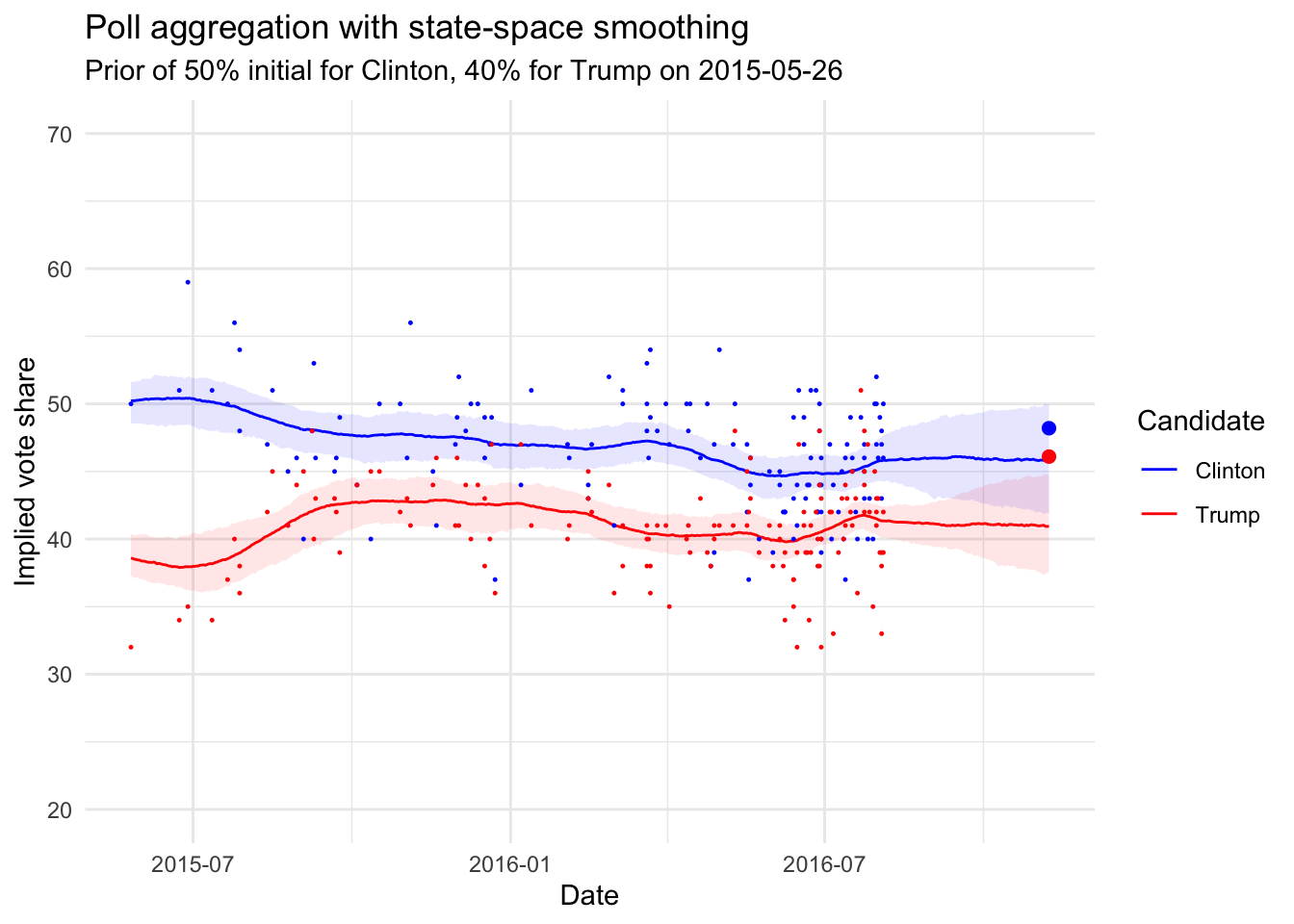
Which gives us the following:

actual_voteshare <- tibble(date = as.Date("2016-11-08"),
                           value = c(48.2, 46.1),
                           candidate = c("Clinton", "Trump"))

bind_rows(mu_ts_clinton, mu_ts_trump) %>%
  ggplot(aes(x = date)) +
  geom_ribbon(aes(ymin = lower, ymax = upper, fill = candidate),alpha = 0.1) +
  geom_line(aes(y = median, colour = candidate)) +
  ylim(20, 70) +
  scale_colour_manual(values = c("blue", "red"), "Candidate") +
  scale_fill_manual(values = c("blue", "red"), guide = F) +
  geom_point(data = polls4, aes(x = end_date, y = `Clinton`), size = 0.2, colour = "blue") +
  geom_point(data = polls4, aes(x = end_date, y = Trump), size = 0.2, colour = "red") +
  xlab("Date") +
  ylab("Implied vote share") +
  ggtitle("Poll aggregation with state-space smoothing",
          subtitle= paste("Prior of 50% initial for Clinton, 40% for Trump on", min(polls4$end_date)))+
  theme_minimal()+
  geom_point(data = filter(actual_voteshare, candidate == "Clinton"),
             aes(date, value), colour = "blue", size = 2)+
  geom_point(data = filter(actual_voteshare, candidate == "Trump"),
             aes(date, value), colour = "red", size = 2)

So the outcome was not totally out of the bounds of a good predictive model!

Citation

BibTex citation:

@online{dewitt2019
author = {Michael E. DeWitt},
title = {State Space Models for Poll Prediction},
date = 2019-05-19,
url = {https://michaeldewittjr.com/articles/2019-05-18-state-space-models-for-poll-prediction},
langid = {en}
}

For attribution, please cite this work as:

Michael E. DeWitt. 2019. "State Space Models for Poll Prediction." May 19, 2019. https://michaeldewittjr.com/articles/2019-05-18-state-space-models-for-poll-prediction