Approval Rating Now?

Posted on September 26^th, 2019

This one is a quick one and based on some work that I have already done. Given the ongoing controversy about President Trump potentially using publically held funds to strong arm a foreign entity for personal and political gain, I figured it was time to do some state-space modeling on approval polls. This will be a quick one just because I want an answer.

The Data

I am going to get some approval polling data from fivethirtyeight. I sincerely appreciate that they put this data out for others to use. Do I wish it had some weights and more data cooked into it? Absolutely. Do I have the resources to do something better? No, I do not. But anyways, thanks fivethirtyeight!

suppressPackageStartupMessages(library(tidyverse))
theme_set(theme_minimal())
dat <- read_csv("https://projects.fivethirtyeight.com/polls-page/president_approval_polls.csv")
base_path <- file.path("posts", "2019-09-26-approval-rating-now")

Multiple Polls on Multiple Days?

In order to build the data for Stan, it is necessary to make some wide data frame. Additionally, I need to calculate some standard errors. Just a reminder for those at home, the standard error for a binomial distribution is:

$SE = \sqrt\frac{p(1-p)}{n}$

I’m also going to use some of the new pivot_* functions from {tidyr}. They are great! These tools bring back some of the functionality that was missing when {tidyr} emerged from {reshape2}.

library(lubridate)
dat_range <- crossing(seq(min(mdy(dat$end_date)),
                 max(mdy("11/1/2019")),
                     "1 day") %>%
  enframe(name = NULL) %>%
  set_names("date_range"), pollster = unique(dat$pollster))

formatted_data <- dat %>%
  mutate(my_end = lubridate::mdy(end_date)) %>%
  select(my_end, yes, sample_size, pollster) %>%
  mutate(polling_var = sqrt(.5 * (1-.5)/sample_size)*100) %>%
  right_join(dat_range, by = c("my_end" = "date_range", "pollster"))

formatted_data[is.na(formatted_data)] <- -9

sigma <- formatted_data %>%
  select(my_end, pollster, polling_var) %>%
  pivot_wider(names_from = pollster,
              values_from = polling_var,
              values_fn = list(polling_var = max)) %>%
  select(-my_end) %>%
  as.matrix()

y <- formatted_data %>%
  select(my_end, pollster, yes) %>%
  pivot_wider(names_from = pollster,
              values_from = yes,
              values_fn = list(yes = max)) %>%
  select(-my_end) %>%
  as.matrix()

Our Model

This is the same model from this blog post courtesy of James Savage and Peter Ellis.

// Base Syntax from James Savage at https://github.com/khakieconomics/stanecon_short_course/blob/80263f84ebe95be3247e591515ea1ead84f26e3f/03-fun_time_series_models.Rmd
//and modification inspired by Peter Ellis at https://github.com/ellisp/ozfedelect/blob/master/model-2pp/model-2pp.R

data {
  int polls; // number of polls
  int T; // number of days
  matrix[T, polls] Y; // polls
  matrix[T, polls] sigma; // polls standard deviations
  real inflator;         // amount by which to multiply the standard error of polls
  real initial_prior;
  real random_walk_sd;
  real mu_sigma;
}
parameters {
  vector[T] mu; // the mean of the polls
  real<lower = 0> tau; // the standard deviation of the random effects
  matrix[T, polls] shrunken_polls;
}
model {
  // prior on initial difference
  mu[1] ~ normal(initial_prior, mu_sigma);
  tau ~ student_t(4, 0, 5);
  // state model
  for(t in 2:T) {
    mu[t] ~ normal(mu[t-1], random_walk_sd);
  }

  // measurement model
  for(t in 1:T) {
    for(p in 1:polls) {
      if(Y[t, p] != -9) {
        Y[t,p]~ normal(shrunken_polls[t, p], sigma[t,p] * inflator);
        shrunken_polls[t, p] ~ normal(mu[t], tau);
      } else {
        shrunken_polls[t, p] ~ normal(0, 1);
      }
    }
  }
}

Prep the Data

Now we can put the data in the proper format for Stan. I’m also going to supply the 2016 voteshare as the initial prior. This is probably a favourable place to start.

library(rstan)
rstan_options(auto_write = TRUE)
options(mc.cores = parallel::detectCores())
approval_data <- list(
  T = nrow(y),
  polls = ncol(sigma),
  Y = y,
  sigma = sigma,
  initial_prior = 46, # 2016 Election Results
  random_walk_sd = 0.2,
  mu_sigma = 1,
  inflator =sqrt(2)
)

Run the Model

Now we can run the model. Caution, this takes a good while to run…oh how I miss having a cluster….

sstrump <- stan_model(file.path(base_path, "sstrump.stan"))
trump_model <- sampling(sstrump,
                    data = approval_data,
                    iter = 1000,
                    refresh = 0,
                    chains = 2,
                    control = list(adapt_delta = .95,
                                     max_treedepth = 15))

Did It Converge?

I’m just going to look quickly at some of the Rhat values. I see that some of my ESS are a little lower than I would like. This isn’t completely surprising given the sparsity of data (57 different polls).

print(trump_model, pars = "mu")

Now Let’s see…

Now we can extract the model fit and see how it looks!

mu_trump <- extract(trump_model, pars = "mu", permuted = T)[[1]] %>%
  as.data.frame

names(mu_trump) <- unique(dat_range$date_range)

mu_ts_trump <- mu_trump %>% reshape2::melt() %>%
  mutate(date = as.Date(variable)) %>%
  group_by(date) %>%
  summarise(median = median(value),
            lower = quantile(value, 0.025),
            upper = quantile(value, 0.975),
            candidate = "Trump")

Partisanship…

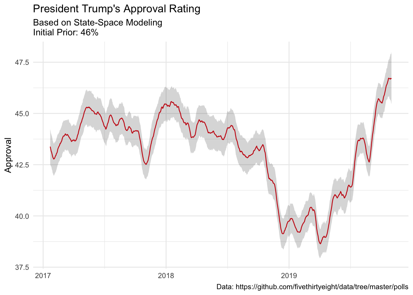
Looks like despite a dip in late 2017, Mr. Trump’s approval rating is remarkably stable (as a reminder, it looks like the lowest ever was 25% for President G.W. Bush). It will be curious to see how this changes as more information comes out regarding Mr. Trumps actions with Ukraine.

mu_ts_trump %>%
  ggplot(aes(date, median))+
  geom_line(color = "#E91D0E")+
  geom_ribbon(aes(ymin = lower, ymax = upper), alpha = .2)+
  labs(
    title = "President Trump's Approval Rating",
    subtitle = "Based on State-Space Modeling\nInitial Prior: 46%",
    caption = "Data: https://github.com/fivethirtyeight/data/tree/master/polls",
    y = "Approval",
    x = NULL
  )+
  geom_vline(xintercept = as.Date(Sys.Date()), color = "orange")

Citation

BibTex citation:

@online{dewitt2019
author = {Michael E. DeWitt},
title = {Approval Rating Now?},
date = 2019-09-26,
url = {https://michaeldewittjr.com/articles/2019-09-26-approval-rating-now},
langid = {en}
}

For attribution, please cite this work as:

Michael E. DeWitt. 2019. "Approval Rating Now?." September 26, 2019. https://michaeldewittjr.com/articles/2019-09-26-approval-rating-now