How About Impeachment?

Posted on October 8^th, 2019

So I suppose this is a logical follow-up to the previous post. Now, instead of approval, we can look at impeachment.

The Data

Our friends at fivethirtyeight have not publically shared the polls that they have aggregated, so I will use my own aggregations.

suppressPackageStartupMessages(library(tidyverse))
theme_set(theme_minimal())
dat <- read_csv("https://gist.githubusercontent.com/medewitt/74ad210ea8cd3e5870e44a8b3b2e7d64/raw/116273bc73830331bd6b8c1fdd9e48d5ccb8cc8d/impeachment.csv")

base_path <- file.path("posts", "2019-10-08-how-about-impeachment")

Multiple Polls on Multiple Days?

In order to build the data for Stan, it is necessary to make some wide data frame. Additionally, I need to calculate some standard errors. Just a reminder for those at home, the standard error for a binomial distribution is:

$SE = \sqrt\frac{p(1-p)}{n}$

As I did last time, I’m also going to use some of the new pivot_* functions from {tidyr}. They are great! These tools bring back some of the functionality that was missing when {tidyr} emerged from {reshape2}. It would probably be better to use the MOE as specified by the pollster to get the true design effect, but just to crank this out, I am not going to do that.

library(lubridate)
dat_range <- crossing(seq(min(dat$date, na.rm = TRUE),
                 max(mdy("11/1/2019")),
                     "1 day") %>%
  enframe(name = NULL) %>%
  set_names("date_range"), pollster = unique(dat$pollster))

formatted_data <- dat %>%
  mutate(my_end = date) %>%
  select(my_end, approve, n = n, pollster) %>%
  mutate(polling_var = sqrt(.5 * (1-.5)/n)*100) %>%
  right_join(dat_range, by = c("my_end" = "date_range", "pollster"))

formatted_data[is.na(formatted_data)] <- -9

sigma <- formatted_data %>%
  select(my_end, pollster, polling_var) %>%
  pivot_wider(names_from = pollster,
              values_from = polling_var,
              values_fn = list(polling_var = max)) %>%
  select(-my_end) %>%
  as.matrix()

y <- formatted_data %>%
  select(my_end, pollster, approve) %>%
  pivot_wider(names_from = pollster,
              values_from = approve,
              values_fn = list(yes = max)) %>%
  select(-my_end) %>%
  as.matrix()

Our Model

This is the same model from this blog post and this one courtsey of James Savage and Peter Ellis.

// Base Syntax from James Savage at https://github.com/khakieconomics/stanecon_short_course/blob/80263f84ebe95be3247e591515ea1ead84f26e3f/03-fun_time_series_models.Rmd
//and modification inspired by Peter Ellis at https://github.com/ellisp/ozfedelect/blob/master/model-2pp/model-2pp.R

data {
  int polls; // number of polls
  int T; // number of days
  matrix[T, polls] Y; // polls
  matrix[T, polls] sigma; // polls standard deviations
  real inflator;         // amount by which to multiply the standard error of polls
  real initial_prior;
  real random_walk_sd;
  real mu_sigma;
}
parameters {
  vector[T] mu; // the mean of the polls
  real<lower = 0> tau; // the standard deviation of the random effects
  matrix[T, polls] shrunken_polls;
}
model {
  // prior on initial difference
  mu[1] ~ normal(initial_prior, mu_sigma);
  tau ~ student_t(4, 0, 5);
  // state model
  for(t in 2:T) {
    mu[t] ~ normal(mu[t-1], random_walk_sd);
  }

  // measurement model
  for(t in 1:T) {
    for(p in 1:polls) {
      if(Y[t, p] != -9) {
        Y[t,p]~ normal(shrunken_polls[t, p], sigma[t,p] * inflator);
        shrunken_polls[t, p] ~ normal(mu[t], tau);
      } else {
        shrunken_polls[t, p] ~ normal(0, 1);
      }
    }
  }
}

Prep the Data

Now we can put the data in the proper format for Stan. I’m also going to supply the 2016 voteshare as the initial prior. This is probably a favourable place to start.

library(rstan)
rstan_options(auto_write = TRUE)
options(mc.cores = parallel::detectCores())
approval_data <- list(
  T = nrow(y),
  polls = ncol(sigma),
  Y = y,
  sigma = sigma,
  initial_prior = 40, # Rough dissapproval ratings
  random_walk_sd = 0.2,
  mu_sigma = 1,
  inflator =sqrt(2)
)

Run the Model

Now we can run the model. This might take a little while, but we have relatively sparse data and few instances per pollster, so it is what it is.

getwd()
sstrump <- stan_model(file.path(base_path, "sstrump.stan"))

trump_model <- sampling(sstrump,
                    data = approval_data,
                    iter = 2000,
                    refresh = 0,
                    chains = 2,
                    control = list(adapt_delta = .99,
                                     max_treedepth = 15))

Did It Converge?

I’m just going to look quickly at some of the Rhat values. I see that some of my ESS are a little lower than I would like. This isn’t completely surprising given the sparsity of data (57 different polls).

summary(trump_model, pars = "mu")$summary[1:15,]

Now Let’s see…

Now we can extract the model fit and see how it looks!

mu_trump <- extract(trump_model, pars = "mu", permuted = T)[[1]] %>%
  as.data.frame

names(mu_trump) <- unique(dat_range$date_range)

mu_ts_trump <- mu_trump %>% reshape2::melt() %>%
  mutate(date = as.Date(variable)) %>%
  group_by(date) %>%
  summarise(median = median(value),
            lower = quantile(value, 0.025),
            upper = quantile(value, 0.975),
            candidate = "Trump")

More to Come

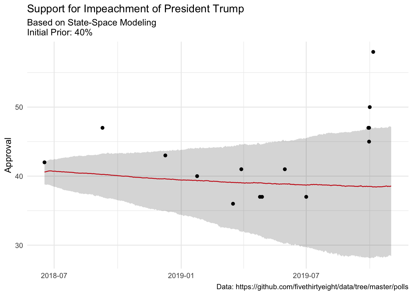
Our model has fairly wide credible intervals, which is to be expected, but the last few point estimates are clear…something is happening. And it looks like something that happened about a week or two has started to move the trend….

mu_ts_trump %>%
  ggplot(aes(date, median))+
  geom_line(color = "#E91D0E")+
  geom_ribbon(aes(ymin = lower, ymax = upper), alpha = .2)+
  labs(
    title = "Support for Impeachment of President Trump",
    subtitle = "Based on State-Space Modeling\nInitial Prior: 40%",
    caption = "Data: https://github.com/fivethirtyeight/data/tree/master/polls",
    y = "Approval",
    x = NULL
  )+
  geom_vline(xintercept = as.Date(Sys.Date()), color = "orange")+
  geom_point(data = dat, (aes(date, approve)))

Citation

BibTex citation:

@online{dewitt2019
author = {Michael E. DeWitt},
title = {How About Impeachment?},
date = 2019-10-08,
url = {https://michaeldewittjr.com/articles/2019-10-08-how-about-impeachment},
langid = {en}
}

For attribution, please cite this work as:

Michael E. DeWitt. 2019. "How About Impeachment?." October 8, 2019. https://michaeldewittjr.com/articles/2019-10-08-how-about-impeachment