Optimisation with Stan

Posted on August 27^th, 2020

In this post I just wanted to play around using the ability to optimize functions in Stan. I know that there are other solvers available, but I just wanted to try this one to start (and I can’t find it now, but I think this was discussed in Regression and Other Stories).

First, I’ll load the cmstanr package which has become my favourite way to interface with Stan.

library(cmdstanr)

Now we can compile a simple optimization scenario which could be a pretty classic production function where you get 2 dollars for widget x and four dollars for wiget y:

$\text{optimize } 2<em>x + 4</em>y \newline \text{subject to:} \newline 0\le x \le 10 \newline 0\le y \le 20 \newline$

There are also contraints on how many units you can make of each.

m <- cmdstan_model(file.path("optim.stan"))

Now print the code:

writeLines(readLines("optim.stan"))

//Test program for optimization

data{

}

parameters{
  real<lower=0,upper=10> x;
  real<lower=0,upper=20> y;
}
model{
  target += 2*x +4*y;
}

Run the model:

fit <- m$sample(refresh = 0)

Summarise the outputs:

fit$print()
out <- fit$draws(inc_warmup = FALSE, variables = c("x", "y"))
out_x <- rowMeans(as.data.frame(out[,,1]))
out_y <- rowMeans(as.data.frame(out[,,2]))

 variable  mean median   sd  mad    q5   q95 rhat ess_bulk ess_tail
     lp__ 94.71  95.06 1.14 0.83 92.35 95.80 1.00     1291     1438
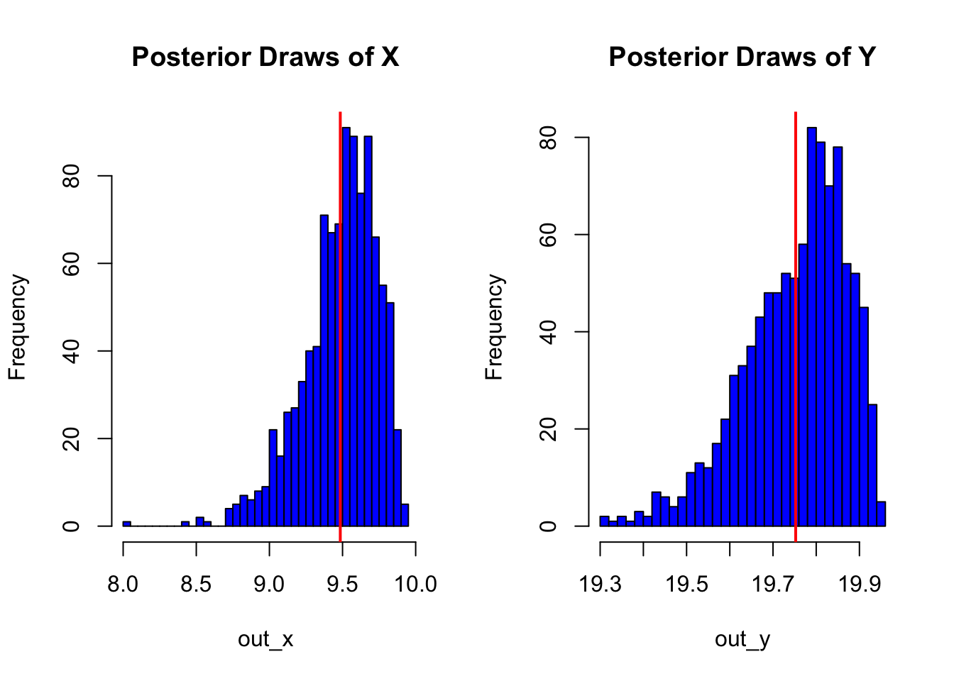
     x     9.48   9.64 0.51 0.36  8.47  9.97 1.00     1771     1099
     y    19.75  19.82 0.24 0.18 19.24 19.99 1.00     1923     1360

Graph the outputs:

op <- par(mfrow = c(1,2))
op
hist(out_x, breaks = 30, main = "Posterior Draws of X", col = "blue")
abline(v = mean(out_x), lwd = 2, col = "red")
hist(out_y, breaks = 30, main = "Posterior Draws of Y", col = "blue")
abline(v = mean(out_y), lwd = 2, col = "red")

Pretty neat that it works.

Alternatively, you could use the optimize function from CmdStan, but this is a bit of a contrite example. More discussion on this is available at this post. Additionally it is important that the target syntax increments the log-density. In our case it doesn’t matter, but in others it might.

A Second Example

Just to play a bit, I want to add some data. Say we have the same function to optimize to maximize revenue, but instead of making any value of x and y, we have some production data with variability. Perhaps these can be real output from our operating process (machines breakdown and life happens, so a higher value might not be reasonable.)

m2 <- cmdstan_model(file.path("optim2.stan"))

Edit 2022-06-02, I realized I didn’t show the code in earlier versions.

writeLines(readLines("optim2.stan"))

//Test program for optimization

data{
  int<lower=1> N; //number of obs
  vector[N] y_in; // observed y
  vector[N] x_in; // observed x
  real<lower=0> sd_y;
  real<lower=0> sd_x;
}

parameters{
  real<lower=0,upper=100> x;
  real<lower=0,upper=200> y;
}
model{
  y_in ~ normal(y, sd_y);
  x_in ~ normal(x, sd_x);

  target += 2*x +4*y;
}

dat <- list(
  y_in = rnorm(100, 7, 1.2),
  x_in = rnorm(100, 23, 5),
  sd_x = 5L,
  sd_y = 2L,
  N = 100L
)

fit2 <- m2$sample(data = dat, refresh = 0)

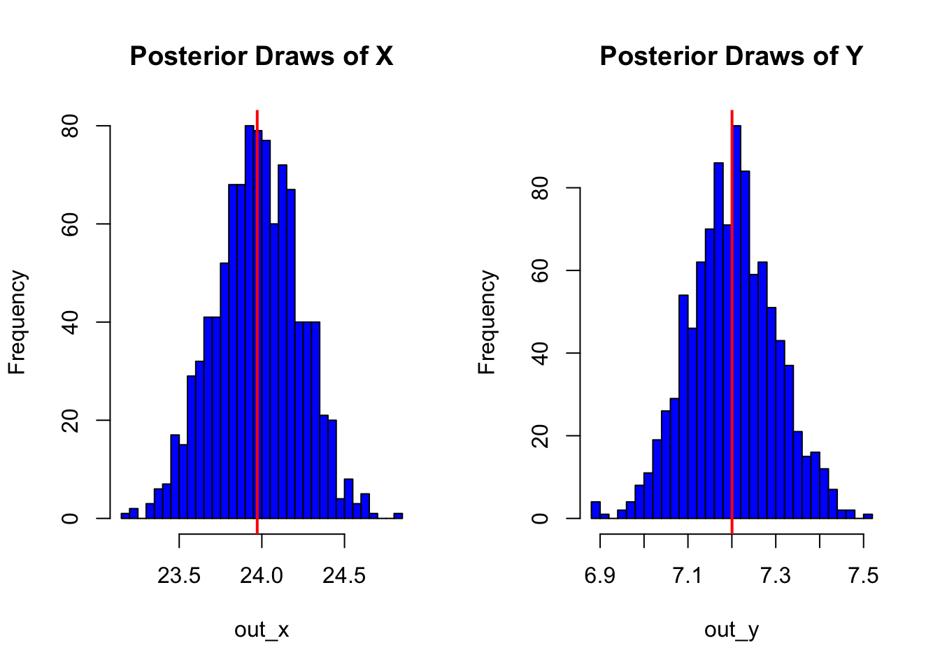
Now we can see the results:

fit2$print()

 variable  mean median   sd  mad    q5   q95 rhat ess_bulk ess_tail
     lp__ 10.53  10.82 0.95 0.70  8.65 11.45 1.00     1854     2462
     x    23.97  23.97 0.50 0.51 23.16 24.79 1.00     3721     2765
     y     7.20   7.20 0.19 0.19  6.88  7.52 1.00     3569     2629

out <- fit2$draws(inc_warmup = FALSE, variables = c("x", "y"))
out_x <- rowMeans(as.data.frame(out[,,1]))
out_y <- rowMeans(as.data.frame(out[,,2]))
op <- par(mfrow = c(1,2))
op
hist(out_x, breaks = 30, main = "Posterior Draws of X", col = "blue")
abline(v = mean(out_x), lwd = 2, col = "red")
hist(out_y, breaks = 30, main = "Posterior Draws of Y", col = "blue")
abline(v = mean(out_y), lwd = 2, col = "red")

The results from the second model represent the influence of the data from our actual manufacturing process. This can be valuable when trying to optimize these kinds of problems when the true data generating process is available to us.

Citation

BibTex citation:

@online{dewitt2020
author = {Michael E. DeWitt},
title = {Optimisation with Stan},
date = 2020-08-27,
url = {https://michaeldewittjr.com/articles/2020-08-27-optimisation-with-stan},
langid = {en}
}

For attribution, please cite this work as:

Michael E. DeWitt. 2020. "Optimisation with Stan." August 27, 2020. https://michaeldewittjr.com/articles/2020-08-27-optimisation-with-stan