• Home
• Contact
• Selected works
• Newsfeed
• About
• Search

library(cmdstanr)
library(magrittr)
library(ggplot2)
library(data.table)
library(deSolve)

Compartment models are commonly used in epidemiology to model epidemics. Compartmental model are composed of differential equations and captured some “knowns” regarding disease transmission. Because these models seek to simulate/ model the epidemic process directly, they are are somewhat more resistant to some biases (e.g. missing data). Strong-ish assumptions must be made regarding disease transmission and varying level of detail can be included in order to make the models closer to reality.

This post is largely an extension of Bayesian workflow for disease transmission modeling in Stan.

Data Generating Process

First we need to define our data generating process. Here we will start with a four compartment model with no births or deaths. This will represent an immunizing infection with a latent phase.

library(DiagrammeR)

a_graph <-
  create_graph(directed = TRUE) %>%
  add_node(label = "S",
           node_aes = node_aes(fill = "orange")) %>%
  add_node(label = "E",
           node_aes = node_aes(fill = "orange")) %>%
  add_node(label = "I",
           node_aes = node_aes(fill = "orange"))%>%
  add_node(label = "R",
           node_aes = node_aes(fill = "orange")) %>%
  add_edge(from = 1, to = 2) %>%
  add_edge(from = 2, to = 3) %>%
  add_edge(from = 3, to = 4)
render_graph(a_graph, layout = "nicely")

Simulate an Epidemic with Knowns

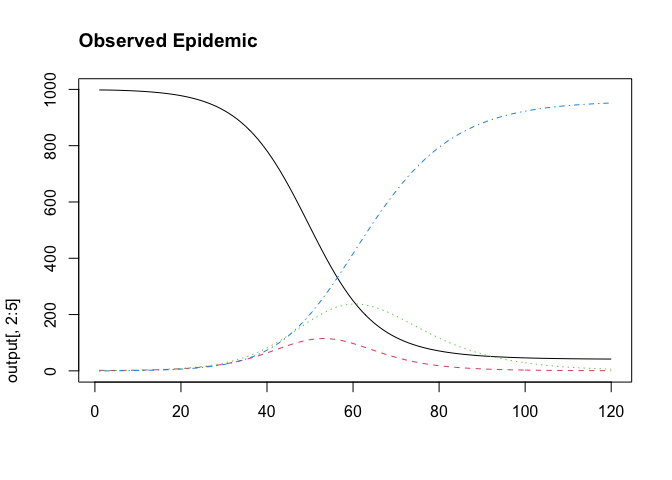
Now we can build this hypothetical epidemic using the “deSolve” package from R. Ideally, we will be able to recover our model parameters using our Bayesian model. This gives us confidence in fitting real data that we observe. This is a key step in the Bayesian workflow where we generate fake data, fit the fake data, and then examine the fit to ensure that we recover the real parameter before we fit our observed data.

seir_model = function (current_timepoint, state_values, parameters)
{
  # create state variables (local variables)
  S = state_values [1]        # susceptibles
  E = state_values [2]        # exposed
  I = state_values [3]        # infectious
  R = state_values [4]        # recovered
  N = state_values [1] + state_values [2] + state_values [3] +state_values [4]

  with (
    as.list (parameters),     # variable names within parameters can be used
         {
           # compute derivatives
           dS = (-beta * S * I)/N
           dE = (beta * S * I)/N - (delta * E)
           dI = (delta * E) - (gamma * I)
           dR = (gamma * I)

           # combine results
           results = c (dS, dE, dI, dR)
           list (results)
         }
    )
}

beta_value <- 1/3
gamma_value <- 1/10
delta_value <- 1/4

parameter_list <- c (beta = beta_value, gamma = gamma_value, delta = delta_value)
times <- 1:120
initial_values <- c(S= 1000-2, E = 2, I =0, R = 0)
output = lsoda (initial_values, times, seir_model, parameter_list)

matplot(output[,2:5], main = "Observed Epidemic", type = "l", adj =0)

We can extract the daily incidence using the following equation. This represents what would typically be reported by authorities. To make it more realistic, it would be good to convolve the cases with a delay distribution to indicate the lag we observe in case reporting. A deconvolution step could then be written into Stan in order to account for this delay distribution.

cases <-  ceiling(output[,2] - shift(output[,2],-1))
cases <- cases[-length(cases)]

Now let’s calculate our basic reproduction number or $R_0$

beta_value/gamma_value

Build Model in Stan

Now we can build the model in Stan as shown below. Ideally, I would write the ODE solver using the new syntax, but I’ll leave that to next time. We can see that the differential equations have been built into the “sir” function.

mod <- cmdstan_model(file.path("sir.stan"))

mod$print()

Build Dataset

Now we can prep our dataset for Stan.

# total count
N <- 1000;

# times
n_days <- length(cases) +1
t <- seq(0, n_days, by = 1)
t0 = 0
t <- t[-1]

#initial conditions
i0 <- 1
e0 <- 0
s0 <- N - i0
r0 <- 0
y0 = c(S = s0, E = e0, I = i0, R = r0)

Run the Model

Then we can run it using CmdStanR.

# number of MCMC steps
niter <- 2000

n_pred <- 21

data_sir<- list(n_days = n_days,
                        y0 = y0,
                        t0 = t0, ts = t,
                        N = N, cases = cases,
                        n_pred = n_pred,delta_mu=.2,
                        ts_pred = seq(n_days+1, n_days+n_pred, by = 1)
                        )

fit <- mod$sample(data = data_sir,
                  adapt_delta = .9,
                  chains = 2,
                  max_treedepth = 12,
                  parallel_chains = 2,
                  iter_sampling = niter/2,
                  refresh = 0,
                  iter_warmup = niter/2)

fit_sir<- rstan::read_stan_csv(fit$output_files())

rstan::extract(fit_sir, "y_pred")->y_pred

str(y_pred)
med_estimates <- colMeans(y_pred[[1]])

Review Model Outputs

Let’s see if we recovered our actual parameters (yes, it appears so)!

pars=c('theta', "R0", "recovery_time")
fit$summary(variables = pars)

Visualise the Epidemic Curve

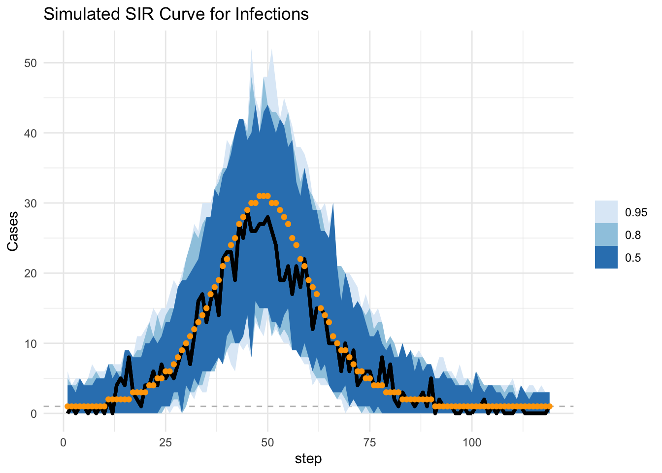
Finally, we can visualise our model outputs and see if we capture our actual cases. Additionally, I am using ggdist to capture the full range of possibilities as discussed in in my previous blog post

library(rstan)
library(ggdist)
library(dplyr)

extract(fit_sir, pars = "pred_cases")[[1]] %>%
  as.data.frame() %>%
  mutate(.draw = 1:n()) %>%
  tidyr::gather(key,value, -.draw) %>%
  mutate(step = readr::parse_number(stringr::str_extract(key,"\newlined+"))) %>%
  group_by(step) %>%
  curve_interval(value, .width = c(.5, .8, .95)) %>%
  ggplot(aes(x = step, y = value)) +
  geom_hline(yintercept = 1, color = "gray75", linetype = "dashed") +
  geom_lineribbon(aes(ymin = .lower, ymax = .upper)) +
  scale_fill_brewer() +
  labs(
    title = "Simulated SIR Curve for Infections",
    y = "Cases"
  )+
  geom_point(data = tibble(cases = cases, t = 1:length(cases)),
             aes(t, cases), inherit.aes = FALSE, colour = "orange")+
  theme_minimal()

Looks like this model adequately captured our fake data! Part 2 will fit some real data.

Citation

BibTex citation:

@online{dewitt2020
author = {Michael E. DeWitt},
title = {Bayesian SIR},
date = 2020-08-28,
url = {https://michaeldewittjr.com/articles/2020-08-28-bayesian-sir},
langid = {en}
}

For attribution, please cite this work as:

Michael E. DeWitt. 2020. "Bayesian SIR." August 28, 2020. https://michaeldewittjr.com/articles/2020-08-28-bayesian-sir