• Home
• Contact
• Selected works
• Newsfeed
• About
• Search

Reading the Pre-Prints

A prominant scientist has been posting his highlights of pre-prints on twitter during the course of the pandemic and occasionally, I come across one that makes me scratch my head. I think that the move to open and rapid science through pre-prints has been good, but not without issues. Review (and open review especially) makes work better and is an important part of science and progress.

One paper that stood out to me was by Suthar et al. (2021) in which the authors look at the neutralizing antibody tires (nAbs) amongst T-cell response in those persons who were vaccinated with the Pfizer SARS-CoV-2 Vaccines (BNT162b2 vaccine). The authors found: “substantial waning of antibody response and T-cell Immunity” in those who were vaccinated. Naturally, this could be concerning because antibodies and T-cells are important in fighting infection and could help us understand the endgame of this first epidemic of SARS-CoV-2 (e.g., vaccine induced reduction of transmission, symptomatic disease, severe outcomes, and associated periodicity given time since last vaccine). However, there is the open question of what is the best correlate of protection (e.g., we know that antibodies wane with time, but the ability to produce antibodies in the face of a new infection from memory B-cells is also very important) (Corbett et al. 2021)

So Look at the Data

As mentioned, along with the bad things about pre-prints (media jumping on sensationalist findings, people seeking acclaim by making bold statements that are not rigorously founded in fact, general review help, etc) is that much of the data are available for secondary analysis. With the article in question, I could find some of the original data analyzed by the authors from a prior publication. We can start to look at these data ourselves:

library(data.table)
library(tidyverse)
theme_set(ggdist::theme_ggdist())
dat <- readxl::read_excel("nAbs.xlsx")

dat %>%
  gather(day, value, -PID, -Gender) %>%
  mutate(day = as.numeric(str_extract(string = day, "\newlined+")))->dat_long

knitr::kable(dat, digits = 1)

So it appears that there are 57 unique participants. Some participants were lost to follow-up and the final date range is kind of wide (90-120 days).

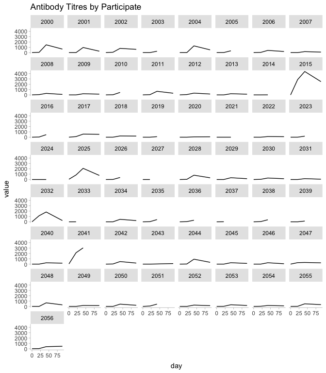
One of the most important steps in any analysis is to graph the data to gain a general understanding of the trends and shape of the data.

dat_long %>%
  ggplot(aes(day, value, group = PID))+
  geom_line()+
  facet_wrap(~PID)+
  labs(
    title = "Antibody Titres by Participate"
  )

One things that stands out to me is participant 2015. This individual has nAbs that are much higher than the other participants.

dat_long %>%
  mutate(tst = ifelse(PID==2015,"PID: 2015","All Others")) %>%
  group_by(tst, day) %>%
  summarise(mu = mean(value, na.rm=TRUE)) %>%
  spread(day,mu) %>%
  knitr::kable(digits = 1, caption = "Mean Value of nAbs by Group")

Mean Value of nAbs by Group

If this were me, I would go back and check those data just in case someone got a little too happy when titrating (been there). Regardless, accepting this level of variability in the individual, these kind of data lend themselves well to hierarchical modeling.

So What’s the Half Life?

We can model the half life of the nAbs in the participants using the multilevel model framework with lme4. I will subset the data to include only the levels after the peak antibody level and include a random effect for the participant (since we know that there is within-person variability and serial dependence).

library(lme4)

fit_lme <- lmer(log(value) ~ day + (1|PID), data = subset(dat_long, day >21))

(half_life <- -log(2)/confint(fit_lme)[4,])

   2.5 %   97.5 %
46.31701 84.74999

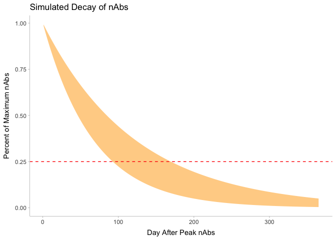
So based on this model, the half-life for nAbs is between 46.3 and 84.7 days.

nab_out <- function(t,hl){
  2^(-t/hl)
}

sim_dat <- tibble(day = 1:365) %>%
  mutate(lower_bound = nab_out(day, half_life[1]),
         upper_bound = nab_out(day, half_life[2]))
sim_dat %>%
  ggplot(aes(x = day))+
  geom_ribbon(aes(ymin = lower_bound,
                  ymax = upper_bound),
              fill = "orange", alpha = .5)+
  geom_hline(yintercept = .25, col = "red", lty = "dashed")+
  labs(
    title = "Simulated Decay of nAbs",
    y  = "Percent of Maximum nAbs",
    x = "Day After Peak nAbs"
  )

So it appears that in roughly 3-6 months after maximum antibody levels a given vaccinated person would have 1/4 of nAb titres.

days_until_perc <- function(target, hl){
  -log(target)*hl/log(2)
}

round(days_until_perc(.25, half_life)/30,1)

 2.5 % 97.5 %
   3.1    5.6

The big question of course is first, does this matter and in what context (protection vs infection where high levels of nAbs make sense vs symptomatic disease where a trained immune system is all that is required (thinking memory B and T cells)) and what concentration is enough at each level.

Is 5% of peak is enough then we have between 6 months and a year, perhaps in time for a teaser from infection to boost nAbs.

round(days_until_perc(.05, half_life)/30,1)

 2.5 % 97.5 %
   6.7   12.2

What about compartmental models?

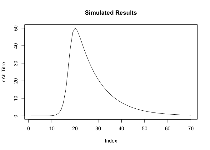
This is not my forte, but it would seem that compartmental models would be a good way to approach this problem. We would have to fix some parameters due to the data available but one could imagine that a decent data generating process could look like (at least as far as I understand how mRNA vaccines work):

1. Inoculum is added to the blood stream via vaccination
2. A latent phase for vaccinated individual’s cells to produce the spike protein which would be a function of the volume of inoculum and the number of cells encountered. The inoculum also has some decay function.
3. A phase where the encoded protein is in the bloodstream and recognized by the immune system as a foreign body which ramps up the innate and humoral immune response.
4. Eventually the spike proteins would be cleared at some rate as the immune response increases

I started down this path and then realized that I would need to make some assumptions for some of the parameters (transition rates between compartments). Being that I do not have reasonable priors for these rates, I decided not to code up this mdoel.

Other Method

I read another paper on waning immunity on coronaviruses that had much more longitudinal data (Townsend et al. 2021). The key model in the paper was locked away in a proprietary Mathematica Notebook that couldn’t open without buying the software. I coded the below model based on their methods, but we will find is that we do not have enough data to fit a very good model.

rw("decay.stan")

data {
    int<lower=1> N; // Number of Samples
    int<lower=1> J; //Number of participants
    vector [N] nAbs; //The concentration of the antibodies
    vector [N] time; //The concentration of the antibodies
}

parameters{
    real omega;
    real hl;
    real<lower=0> sigma;
}

transformed parameters {
    vector[N] theta;  //vac effect
    theta[1:N] = omega + (1- omega)  * exp(-hl*time[1:N]);
}

model {
    hl ~ normal(0,2);
    omega ~ normal(0,1);
    nAbs ~ normal(theta, sigma);
}

library(cmdstanr)

mod_ex <- cmdstan_model("decay.stan")

dat_stan_base <- dat_long %>%
  filter(!is.na(value)) %>%
  filter(day>21)

stan_dat <- list(
  N = nrow(dat_stan_base),
  J = length(unique(dat_stan_base$PID)),
  nAbs = dat_stan_base$value,
  time = dat_stan_base$day
)

fit_ex <- mod_ex$sample(stan_dat,
                        refresh = 0, iter_sampling = 500,
                                                iter_warmup = 200,
                        adapt_delta = .98,
                        max_treedepth = 15)

Running MCMC with 4 parallel chains...

Chain 2 finished in 0.4 seconds.
Chain 4 finished in 0.3 seconds.
Chain 1 finished in 0.8 seconds.
Chain 3 finished in 1.3 seconds.

All 4 chains finished successfully.
Mean chain execution time: 0.7 seconds.
Total execution time: 1.7 seconds.

Not a great fit as we are trying to draw a complicated curve through basically two points and there are (infinitely) many ways to do this.

fit_ex$summary(variables = c("omega", "hl", "sigma"))

# A tibble: 3 × 10
  variable    mean median      sd   mad     q5     q95  rhat ess_bulk ess_tail
  <chr>      <num>  <num>   <num> <num>  <num>   <num> <num>    <num>    <num>
1 omega     -0.624  -1.09   0.940 0.873 -1.68    0.627  2.01     5.95     16.0
2 hl        -0.789  -1.22   1.12  0.438 -1.65    1.97   3.96     4.35     11.5
3 sigma    198.      2.06 341.    1.74   0.217 836.     3.56     4.42     11.1

Viral Titre?

A model that is somewhat of a compromise between the compartmental model which captures more of the underlying biological process and the hierarchical model which fit the within-host variability is to model the viral decay with a direct functional form. This is similar to the approach performed by Singanayagam et al. (2021) who use this functional form for estimated RNA copies from Cycle Threshold values. The issues, as before, is that we only have a few observations per person and I don’t have strong priors, but this model is closer to what we see in the graphs where the titre increases to some point and then decay afterwards. Ideally we would have some additional measures for the participants.

This can be modeled by the following equations:

$$v(\tau) = v_{max} \frac{(a+b)}{be^{-a(\tau-\tau_{max})}+ae^{b(\tau-\tau_{max})}}$$

The a and b parameters can be fit and influence the rate of increase and decrease of nAb tire (or virus titre for that matter).

nab_kinetics <- function(v_max, a,b,t,tmax){
  v_max * (a+b)/(b*exp(-a*(t-tmax))+a*exp(b*(t-tmax)))
}

plot(nab_kinetics(50, a = .8, b= .1, t = 1:70, tmax = 20), type = "l",
     ylab = "nAb Titre", main = "Simulated Results")

We need to comport our data to provide the ability to identify the individual maximums and times for each participant.

long_model_dat <- dat_long %>%
    filter(!is.na(value)) %>%
    group_by(PID) %>%
    mutate(v_max = max(value)) %>%
    mutate(t_max =  max((v_max == value)*day))%>%
    ungroup() %>%
    mutate(id = as.integer(as.factor(PID)))

And our model:

rw("rise.stan")

functions{
    real viral_kinetics (real v_max, real a, real b, real t, real t_max){
        return(v_max * (a + b) / (b * exp(-a*(t - t_max)) + a * exp(b*(t-t_max))));
    }
}

data {
    int<lower=1> N; // Number of records
    int<lower=0> id[N]; //Participant IDs
    vector<lower=0> [N] nAbs_max; // Maximum Ab concentration
    vector<lower=0> [N] nAbs; //The concentration of the antibodies
    vector [N] time; //The concentration of the antibodies
    vector [N] t_max; //The concentration of the antibodies
    real prior_a_mu;
    real prior_b_mu;
    real prior_a_sd;
    real prior_b_sd;
    int pred_window;
}

parameters {
    real<lower=0> a;
    real<lower=0> b;
    real<lower=0> sigma;
}

transformed parameters{
    vector<lower=0>[N] mu;

    for( i in 1:N){
        mu[i] = viral_kinetics(nAbs_max[id[i]], a, b, time[id[i]], t_max[id[i]]);
    }

}
model {
    a ~ normal(prior_a_mu, prior_a_sd);
    b ~ normal(prior_b_mu, prior_b_sd);
    sigma ~ normal(0,1);

    nAbs ~ normal(mu, sigma);
}

generated quantities{
    vector[pred_window] yhat;
    vector[pred_window] mu_pred;
    real avg_nabs_max = mean(nAbs_max);
    real avg_tmax = mean(t_max);

    for(i in 1:pred_window){
        mu_pred[i] = viral_kinetics(avg_nabs_max, a, b, i, avg_tmax);
        yhat[i] = normal_rng(mu_pred[i], sigma);
    }

}

We can fit the model in the usual ways:

mod_titre <- cmdstan_model("rise.stan")

titre_dat <- list(
    N = nrow(long_model_dat),
    id = long_model_dat$id,
    nAbs_max = long_model_dat$v_max,
nAbs = long_model_dat$value,
    time= long_model_dat$day,
    t_max = long_model_dat$t_max,
    prior_a_mu = .8,
    prior_b_mu = .1,
    prior_a_sd = .05,
    prior_b_sd = .05,
pred_window = 180
)

set.seed(336)

fit_titre <- mod_titre$sample(data = titre_dat,
                                                            refresh = 0, adapt_delta = .99,
                                                            max_treedepth = 15)

Running MCMC with 4 parallel chains...

Chain 4 finished in 4.0 seconds.
Chain 1 finished in 4.2 seconds.
Chain 2 finished in 4.2 seconds.
Chain 3 finished in 4.6 seconds.

All 4 chains finished successfully.
Mean chain execution time: 4.2 seconds.
Total execution time: 4.8 seconds.

fit_titre$summary(variables = c("a", "b", "sigma"))

# A tibble: 3 × 10
  variable   mean median     sd    mad      q5    q95  rhat ess_bulk ess_tail
  <chr>     <num>  <num>  <num>  <num>   <num>  <num> <num>    <num>    <num>
1 a         0.800  0.800 0.0505 0.0505  0.718   0.883  1.00    2327.    2255.
2 b         0.102  0.101 0.0460 0.0479  0.0297  0.179  1.00    1706.     980.
3 sigma    91.9   91.9   0.494  0.498  91.1    92.7    1.00    2905.    1739.

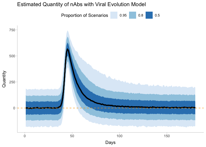
Note that there is a fair bit of variance in our model represented by zero. Additionally, we have some values of the predicted titre below zero. We could resolve this by changing the distribution to use a distribution that is always positive like a lognormal distribution. This would require some careful transformation of our data and associated parameters. We’ll stick with this formulation for now.

We can now visualize our results from this model.

library(posterior)
library(ggdist)
 pred_nab <- tidybayes::gather_draws(fit_titre$draws(variables = "yhat"),yhat[i] ) %>%
    dplyr::ungroup() %>%
    dplyr::group_by(i) %>%
    ggdist::median_qi(.value, .width = c(.5, .8, .95))


pred_nab %>%
    ggplot(aes(i, .value))+
    geom_lineribbon(aes(ymin = .lower, ymax = .upper))+
    scale_fill_brewer()+
    labs(
        title = "Estimated Quantity of nAbs with Viral Evolution Model",
        y = "Quantity",
        x = "Days",
        fill = "Proportion of Scenarios"
    )+
    geom_hline(yintercept = 0, col = "orange", lty = "dashed")+
    theme(legend.position = "top")

Again, we see evidence of detectable tire above 180 days, but there is a decent bit of variability.

Conclusions

If we had additional measurements per person and some additional information on the kinetics, In the time it took me to write this post several other papers have come out with much more information that would be fun to analyze that find that immunity is likely long lasting (Mateus et al., n.d.; Grifoni et al. 2021).

Citation

BibTex citation:

@online{dewitt2021
author = {Michael E. DeWitt},
title = {Neutralizing Antibody Titres},
date = 2021-11-11,
url = {https://michaeldewittjr.com/articles/2021-10-11-neutralizing-antibody-titres},
langid = {en}
}

For attribution, please cite this work as:

Michael E. DeWitt. 2021. "Neutralizing Antibody Titres." November 11, 2021. https://michaeldewittjr.com/articles/2021-10-11-neutralizing-antibody-titres