• Home
• Contact
• Selected works
• Newsfeed
• About
• Search

As the parent to a child under the age of five, I have been anxiously awaiting news regarding the availability of a vaccine against COVID-19 for some time. The news recently was that the FDA was encouraging Pfizer/BioNTech to submit the data for their clinical trials for their vaccine candidate for the 6 month to five year old group. Early reporting was that the vaccine wasn’t meeting it’s endpoints with two doses (which were reduced in concentration from the older groups for fear of vaccine induced myocarditis) and would need to pursue a third dose.

It would appear that once the independent review board looked at the initial data they balked and are now holding off until the results of the April submission.

Only a Bayesian Can Save Us Now

This post really was stirred by Lucy D’Agostino McGowan’s twitter post as shown below. Bayesian analysis allows us to include prior information. It would seem that a clinical trial in the midst of:

• Massive vaccinations across the world
• Continuous evaluation of vaccine efficiency (a la the United Kingdom amongst others)
• New variants which are antigenically different that the lineages on which the vaccines were based

…should take advantage of Bayesian data analysis.

Reviving a Prior Analysis

I am going to take code from a prior blogpost where Bayesian analysis was used to look at Paxlovid, another Pfizer product.

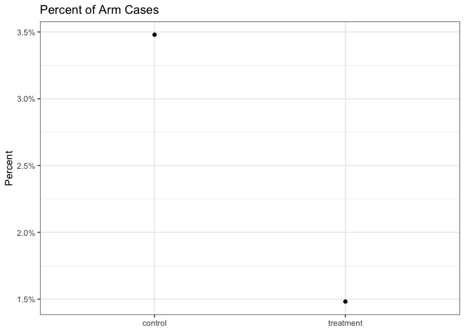
First we visualize our data using the approximations that Dr McGowan gave us:

library(cmdstanr)
library(tidybayes)
library(posterior)
library(ggplot2)
library(dplyr)
library(ggdist)
theme_set(theme_bw())
dat_trials <- tibble::tribble(
  ~"cases", ~"arm_n", ~"arm",
  23, 1552, "treatment",
  27, 776, "control"

) %>%
  mutate(prop = cases/arm_n)


dat_trials %>%
  ggplot(aes(arm, prop))+
  geom_point()+
  scale_y_continuous(labels = scales::percent)+
  labs(
    title = "Percent of Arm Cases",
    y = "Percent",
    x = NULL
  )

We can also calculate the frequentist confidence intervals:¹

ARV <- 23/1552; ARU <- 27/776

RR <- ARV/ARU

(VE <- 1 - RR)

[1] 0.5740741

bounds <- data.frame(upper = exp(log(RR) + 1.96 * sqrt((1-ARV)/23 +(1-ARU)/27)),
lower = exp(log(RR) - 1.96 * sqrt((1-ARV)/23 +(1-ARU)/27)),
VE = VE) %>%
    select(VE, lower, upper)

bounds %>%
    knitr::kable(digits = 2)

Yikes, so based on these frequentist statistics, the Pfizer vaccine fails.

Enter Bayes

Pfizer initially used Bayesian data analysis on their original submission for the 18 and older vaccine. I think it would be worthwhile to re-examine these data under similar priors and see what our results indicate. First we can recycle our previous trial code which considers our prior on the relative risk as well as calculates the net effect.

writeLines(readLines("trial.stan"))

//based on https://www.robertkubinec.com/post/vaccinepval/
// Which is based on https://rpubs.com/ericnovik/692460
data {
  int<lower=1> r_c; // num events, control
  int<lower=1> r_t; // num events, treatment
  int<lower=1> n_c; // num cases, control
  int<lower=1> n_t; // num cases, treatment
  array[2] real a;   // prior values for treatment effect

}
parameters {
  real<lower=0, upper=1> p_c; // binomial p for control
  real<lower=0, upper=1> p_t; // binomial p for treatment
}
transformed parameters {
  real RR  = 1 - p_t / p_c;  // Relative effectiveness
}
model {
  (RR - 1)/(RR - 2) ~ beta(a[1], a[2]); // prior for treatment effect
  r_c ~ binomial(n_c, p_c); // likelihood for control
  r_t ~ binomial(n_t, p_t); // likelihood for treatment
}
generated quantities {
  real effect   = p_t - p_c;      // treatment effect
  real log_odds = log(p_t / (1 - p_t)) - log(p_c / (1 - p_c));
}

Exploring Priors

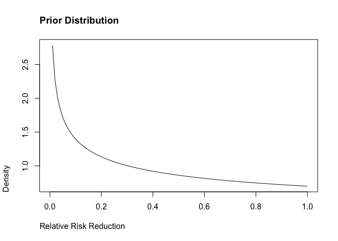
Pfizer initially used some pretty weak, pessimistic priors. The bulk of the distribution is < 0.2, which would indicate that the vaccine is not effective. We can start with these and see what happens.

curve(dbeta(x, shape1 = .700102, shape2 = 1),
      from = 0, to = 1,
      ylab = "Density", xlab = "Relative Risk Reduction",
      main = "Prior Distribution", adj = 0)

It is also interesting to look numerically where the bulk of the distribution lies (which in this case is very wide):

qbeta(p = c(.05,.95), .700102, 1)

[1] 0.01385659 0.92935409

Let’s fit the model:

mod <- cmdstan_model(file.path("trial.stan"))

dat <- list(
  n=sum(dat_trials$arm_n),
       r_c=dat_trials[2,]$cases,
       r_t=dat_trials[1,]$cases,
       n_c=dat_trials[2,]$arm_n,
       n_t=dat_trials[1,]$arm_n,
       a=c(.700102,1)
)
fit <- mod$sample(dat, refresh = 0)

Running MCMC with 4 sequential chains...

Chain 1 finished in 0.0 seconds.
Chain 2 finished in 0.0 seconds.
Chain 3 finished in 0.0 seconds.
Chain 4 finished in 0.0 seconds.

All 4 chains finished successfully.
Mean chain execution time: 0.0 seconds.
Total execution time: 0.6 seconds.

I’m going to write a quick helper function for summarising results from the fitted model.

pull_cis <- function(x){
    x$draws(variables = "RR") %>%
    as_draws_df() %>%
    summarise(mean = mean(RR),
                        median = median(RR),
                        q025 = quantile(RR, 0.025),
                        q975 = quantile(RR, 0.975)) %>%
    mutate(variable = "RR") %>%
    select(variable, mean, median, contains("q")) %>%
    knitr::kable(digits = 2)
}

Using these initial priors we get the following results:

pull_cis(fit)

These don’t look too bad! The 95% credible intervals are similar, though a nudge higher, than the frequentist confidence intervals

Let’s see if we hit the lower endpoint of 30% risk reductions (and really what fraction of the draws are greater than 30%).

draws <- fit$draws(variables = "RR") %>%
    as_draws_df()
mean(as.numeric(draws$RR>.3))

[1] 0.96775

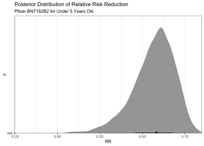
So that’s a bit interesting in that there is a 96.8% posterior probability that the vaccine efficiency is greater than 30% (which is the lower limit of approval). Additionally, there is a 74% posterior probability given these data that the vaccine efficiency (relative risk reduction) is greater than 50%

We can graph these results to display the same information visually.

draws %>%
  #median_qi(VE, .width = c(.5, .89, .995)) %>%
  ggplot(aes(y = "RR", x = RR)) +
  stat_halfeye()+
  scale_color_brewer()+
  coord_cartesian(expand = FALSE)+
  labs(
    title = "Posterior Distribution of Relative Risk Reduction",
    subtitle = "Pfizer BNT162B2 for Under 5 Years Old"
  )

So What?

One key point is that these raw data are inferred from the reporting that there were around 50 cases so these are crude approximations. Regardless this analysis shows that we shouldn’t throw the proverbial baby out with the bathwater. This looks like a vaccine that would meet the endpoints and is showing expected effectiveness given the changing terrain of the pandemic. Of course there are other competing concerns out there–like if a booster is needed would this EUA interrupt that process? Would an EUA cause people to doubt the process (honestly the FDA messed this one up going back and forth with Pfizer on this)? Are there data that have yet to be made public (e.g., faster nAbs waning)? Regardless, this analysis shows that being a Bayesian in these contexts is likely warranted.

Note: Edited 2022-02-12 for typos (per paragraph 1)…

Note2: Moved Bayesian credible intervals to 95% to be consistent with frequentist 95% CIs- Thanks @statstaci5.

Note3: Correct hospitalizations to cases. I have hospitalizations on the brain most of the time. Thanks @LucyStats!

I really need to open up this github repo for this reason but alas….

Citation

BibTex citation:

@online{dewitt2022
author = {Michael E. DeWitt},
title = {Pfizer BNT162b2 for Under 5s},
date = 2022-02-11,
url = {https://michaeldewittjr.com/articles/2022-02-11-pfizer-bnt162b2-for-under-5s},
langid = {en}
}

For attribution, please cite this work as:

Michael E. DeWitt. 2022. "Pfizer BNT162b2 for Under 5s." February 11, 2022. https://michaeldewittjr.com/articles/2022-02-11-pfizer-bnt162b2-for-under-5s