Turing and ODEs
Posted onExploring Julia and ODEs
This post is exploring the use of Julia, Turing, and ODEs and largely expands on the work from Simon Frost’s awesome epirecipes.
Getting Started with Julia
- Julia as a statistical programming language/environment has some really neat properties.
-
::{.column-margin} Speed, generally speed. :::
Turing also has some neat elements when it comes to probabilistic computing/programming. The key feature that interests me is the ability to switch between sampling approaches (e.g., Gibbs, Hamiltonian Monte Carlo, no u-turn sampling, sequential) while keeping the same syntax and model structure. While I absolutely love Stan and have spent many hours learning and the syntax (and it is actively developed, highly optimized, etc), I sometimes wish I could explore other sampling approaches due to strange posteriors (especially when it comes to times when SMC might be better).
The Approach
This is a pretty vanilla post, in which we will first create some fake data from a known distribution and then fit said data. As always, we will bring in the required packages.
using
using
using
using
using
using
Now we can generate a simple three compartment model, with S (susceptibles), I, (infected), and R (recovered).
Additionally:
- On average 10 contacts are made per day
- The contact rate is 0.05 (probability of passing infection to any given contact)
- Those who are infected recover on average every 5 days
- Immunity lasts for a 180 days on average before people become susceptible again
- Population size of 6,000 individuals
- Standard mass-action approach
Something that looks like the following:
using
using
.
.
.
.
.
.
.
.
= 30
= 40
= 6
= -2
.
true

;
= 365.0
=
= 1.0:1.0:
= # S,I.R,C
= ; # β, c, γ, δ
= ;
= ;
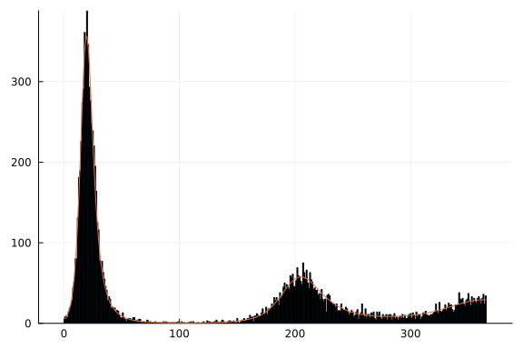
We can then visualize our expected cases:
= # Cumulative cases
= - ;
.
= .;

Note the second wave of cases occuring as immunity begins to wane.
Solve Using Turing
Now we build our model in Turing, using our prior defined ODE. Note that I included a check on the ODE output to try and catch values less than one, otherwise the sampler would reject the solution (because Poisson distributions cannot have a rate parameters less than 0).
= begin
# Calculate number of timepoints
=
~
~
~
= *6000.0
=
=
=
=
=
= # Cumulative cases
= -
=
for in 1:
~
end
end;
= ;
= ;
2-element Vector{MCMCChains.ChainDataFrame}:
 Summary Statistics (3 x 8)
 Quantiles (3 x 6)
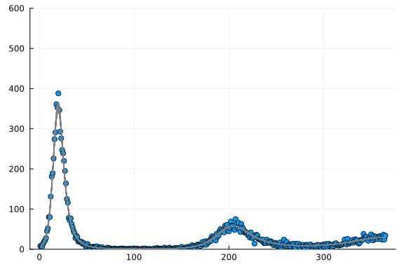
Now let’s see if we were able to recover our parameters:
= ;
=
=
Estimate for  β: 0.04985109789038826
Estimate for immunity duration: 178.3573980140202
Estimate for initial proportion infected: 0.0016206929584588728
Not too bad! Now we can simulate the dynamics going forward:
;
=
for in 1:365
=
end

Conclusions
This shows a very intuitive approach towards compartmental modeling in a Bayesian framework using Julia.
Citation
BibTex citation:
@online{dewitt2022
author = {Michael E. DeWitt},
title = {Turing and ODEs},
date = 2022-08-13,
url = {https://michaeldewittjr.com/articles/2022-08-13-turing-and-odes},
langid = {en}
}
For attribution, please cite this work as:
Michael E. DeWitt. 2022. "Turing and ODEs." August 13, 2022. https://michaeldewittjr.com/articles/2022-08-13-turing-and-odes