Back-Calculation and Deconvolution of Infection Curves

We almost never observe infections directly. Intuitively, it hard to know when an infection began even in a person. Was it the moment that they shared a room with another infected person? Or was it a few hours later into the contact when they rubbed their eyes? If and when they go and seek care, was it only when they started to show symptoms? Did they seek care during the prodrome or during a period with much more pronounced symptoms? Add on to this the delays from testing to result, test result to reported result, and the subsequent potential downstream events (hospitilization, death) and you see that we are dealing with a series of delays that can influence our understanding of how long each of these events takes.

Often official reports are generated from things that are easily (and often unambiguously) countable such as number of new onset hospitalizations per day or number of deaths recorder per day, but what we really want is the true infectious incidence without all the delays that are cooked into these later reports. Back-calculation is the inverse problem of reconstructing the infection curve from the observed reports, given the distribution of that delay. Initially, this aproach was developed to estimate the hidden HIV epidemic from AIDS diagnoses years after infection, and the same machinery now reconstructs infection incidence for any pathogen where a delay separates infection from observation.

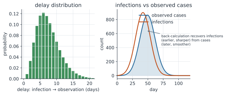
The convolution that links infections and cases#

If $I(s)$ is the number of infections on day $s$ and $f(d)$ is the probability that the observed event follows infection by a delay of $d$ days, then the expected observed count on day $t$ is a convolution,

$$C(t) = \sum_{s \le t} I(s)\, f(t - s).$$

Each day’s cases are a blurred, delayed mixture of infections from earlier days, weighted by the delay distribution. The forward direction is easy: given infections and the delay, you can predict cases. The right panel of the figure shows the effect — the case curve is shifted later and smoothed relative to the infections, with its peak pushed back by roughly the mean delay.

Why inverting it is hard#

Back-calculation runs this backward: given $C(t)$ and $f(d)$, solve for $I(s)$. This is deconvolution, and it is ill-posed (i.e., there are virtually infinitely many possibilities to generate the time series, without making some stronger assumptions about things). The convolution smooths away fine detail, so many different infection curves are consistent with the same observed cases, and a naive inversion amplifies noise into wild oscillations. Every practical method therefore adds regularization — a smoothness penalty, a parametric shape for $I(s)$, or a prior — to select a plausible infection curve among the many that fit (Goldstein et al. 2009, doi:10.1073/pnas.0902958106). The reconstruction is most uncertain at the recent end, where the infections that will produce future cases have not yet been observed, exactly the right-truncation problem that nowcasting addresses.

Back-calculation, nowcasting, and R_t#

These three tasks are the same convolution read three ways. Back-calculation recovers past infections from past cases, deblurring the delay. Nowcasting fills in the not-yet-reported recent cases, correcting right truncation before the curve is complete. Estimating the reproduction number then works on the reconstructed infection or onset curve, because inferring transmission from the raw, delayed case curve puts the turning points in the wrong place. Getting the infection timing right is what keeps a estimated $R_t$ from lagging the epidemic it is meant to track, which is precisely when decisions are made.

A worked example#

We take a known infection curve and a gamma-shaped delay distribution, convolve them to produce the observed cases, and confirm that the case peak lags the infection peak. The forward step is what a back-calculation method inverts.

In code#

R#

days <- 0:80
infections <- 100 * dgamma(days, shape = 6, rate = 0.35)   # a latent wave

d <- 0:21
delay <- dgamma(d, shape = 5, scale = 1.6)
delay <- delay / sum(delay)          # normalized delay distribution

cases <- as.numeric(stats::filter(infections, delay, sides = 1))
cases[is.na(cases)] <- 0

c(infection_peak_day = which.max(infections) - 1,
  case_peak_day      = which.max(cases) - 1)

Python#

import numpy as np
from scipy import stats

days = np.arange(0, 81)
infections = 100 * stats.gamma.pdf(days, a=6, scale=1 / 0.35)  # latent wave

d = np.arange(0, 22)
delay = stats.gamma.pdf(d, a=5, scale=1.6)
delay = delay / delay.sum()          # normalized delay distribution

cases = np.convolve(infections, delay)[: days.size]

print(f"infection peak day = {infections.argmax()}")
print(f"case peak day      = {cases.argmax()}")
print(f"lag introduced     = {cases.argmax() - infections.argmax()} days")

infection peak day = 14
case peak day      = 23
lag introduced     = 9 days

Julia#

using Distributions

days = 0:80
infections = 100 .* pdf.(Gamma(6, 1 / 0.35), days)   # latent wave

d = 0:21
delay = pdf.(Gamma(5, 1.6), d)
delay ./= sum(delay)                 # normalized delay distribution

cases = [sum(infections[max(1, t - length(delay) + 1):t] .*
             reverse(delay[1:min(t, length(delay))])) for t in 1:length(infections)]

(infection_peak_day = argmax(infections) - 1, case_peak_day = argmax(cases) - 1)

Why it matters#

Acting on the case curve when you mean to act on the infection curve builds in a delay-length lag, so back-calculation is what lets analysis reflect when transmission actually happened rather than when it surfaced. Its central lesson is that deconvolution is ill-posed: the observed data pin down the infection curve only loosely, and any reconstruction leans on a smoothness assumption that should be stated and stress-tested. Understanding back calculation as a tool to recover the actual infection rate is important when desiging control measures and understanding the rate of new cases.

Related#

• Nowcasting and Reporting Delays — the right-truncation counterpart at the present
• Fitting Delay Distributions: Truncation and Censoring — estimating the delay $f(d)$ itself
• Epidemiological Intervals and Delays — the biology of the delays being deconvolved
• The Renewal Equation — the forward convolution linking incidence and transmission
• The Effective Reproduction Number and Forecasting — estimated on the reconstructed curve