Severity: Estimating the CFR and IFR During an Outbreak
How deadly is this pathogen is one of the first questions asked in an outbreak and one of the hardest to answer while it is still unfolding. The obvious calculation — deaths divided by cases — is biased, sometimes badly, for reasons that have nothing to do with the pathogen and everything to do with the timing and completeness of what we have observed so far. Getting severity right means separating two different ratios and correcting for the fact that, mid-epidemic, most cases have not yet reached their outcome.
Two ratios: CFR and IFR#
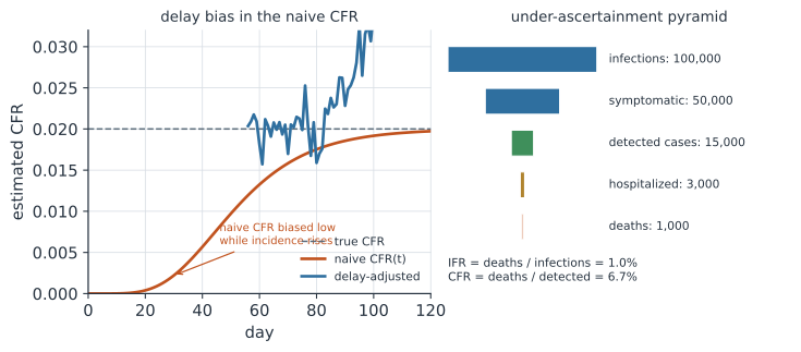
The case fatality ratio (CFR) is the probability of death among detected cases. The infection fatality ratio (IFR) is the probability of death among all infections, including the mild and asymptomatic ones that never become cases. Because only a fraction of infections are ever ascertained, the IFR is always smaller than the CFR, often by a large factor, as the ascertainment pyramid in the figure shows. Which one you want depends on the question: the CFR speaks to the clinical burden among diagnosed patients, while the IFR is what you need to project total deaths from an estimate of total infections. Conflating them, or comparing a CFR from one setting with an IFR from another, is a common and consequential error.
Why the naive CFR is biased mid-epidemic#
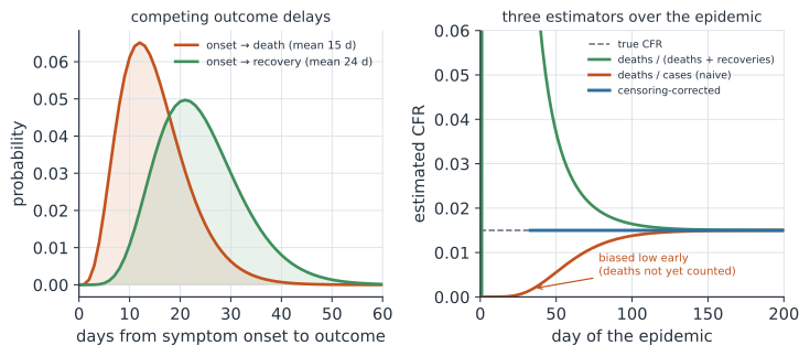
Divide cumulative deaths by cumulative cases during a growing epidemic and you will underestimate the CFR. The reason is right-censoring: a case reported today has not yet had time to die, because death follows symptom onset by a distribution of delays with a mean of two to three weeks. The deaths that these recent cases will eventually contribute are still in the future, so the numerator lags the denominator, and the naive ratio is dragged down. The bias is worst exactly when the epidemic is growing fastest and decision-makers most need the number; it disappears only after the epidemic ends and every case has resolved.
A tempting fix — divide deaths by resolved cases, deaths over deaths-plus-recoveries — overcorrects in the opposite direction. Early in an outbreak, deaths resolve sooner than recoveries because the onset-to-death delay is shorter than the onset-to-recovery delay, so among the cases that have reached an outcome, deaths are over-represented and this ratio runs too high. The two naive estimators bracket the truth, and neither is right until the outbreak is over.
The Ghani/Nishiura correction#
The way out is to put the delay distribution into the estimator directly. Ghani et al. (2005) framed the real-time CFR as a problem of estimating the denominator: not all reported cases have had the chance to die, so the ratio should divide deaths by the number of cases whose outcome would already be known. If is the number of cases with onset on day and is the cumulative distribution of the onset-to-death delay, then by day the expected number of cases with a resolved fatal outcome is
and the corrected estimator is , with the deaths observed so far. Dividing by rather than the raw case count removes the censoring bias, so the estimate tracks the true CFR from early in the epidemic rather than converging to it only at the end.
This same censoring logic drove the influential early COVID-19 severity estimates. The Kucharski group applied it to the closed, near-completely-tested outbreak on the Diamond Princess to pin down an age-adjusted CFR and IFR (Russell et al. 2020), and Verity et al. (2020) combined the delay-adjusted CFR with an age model and an assumed attack rate to produce the widely used early IFR estimate of about 0.66%. The lesson from all three is the same: a severity number reported during an outbreak is meaningless without stating how censoring was handled.
The corrected CFR in code#
We simulate an epidemic with a known true CFR, take a snapshot partway through while it is still growing, and compare the naive and censoring-corrected estimates.
R#
true_cfr <- 0.015
days <- 0:100
cases <- round(2000 * dlnorm(days, meanlog = log(40), sdlog = 0.40))

# Onset-to-death delay distribution and its CDF.
d <- 0:60
f_death <- dgamma(d, shape = 5, scale = 3); f_death <- f_death / sum(f_death)
F_death <- cumsum(f_death)

Tsnap <- 45                                   # snapshot mid-growth
deaths_by_day <- true_cfr * head(
  as.numeric(stats::filter(cases, f_death, sides = 1)), length(days))
deaths_by_day[is.na(deaths_by_day)] <- 0

D <- sum(deaths_by_day[1:(Tsnap + 1)])        # deaths observed so far
naive <- D / sum(cases[1:(Tsnap + 1)])        # deaths / cases
u <- sum(sapply(0:Tsnap, function(s) cases[s + 1] * F_death[Tsnap - s + 1]))
corrected <- D / u                            # deaths / known-outcome cases

round(c(true = true_cfr, naive = naive, corrected = corrected), 4)
Python#
import numpy as np
from scipy import stats

true_cfr = 0.015
days = np.arange(0, 101)
cases = np.round(2000 * stats.lognorm(s=0.40, scale=40).pdf(days))

# Onset-to-death delay distribution and its CDF.
d = np.arange(0, 61)
f_death = stats.gamma(a=5, scale=3).pdf(d)
f_death /= f_death.sum()
F_death = np.cumsum(f_death)

Tsnap = 45                                       # snapshot mid-growth
deaths_by_day = true_cfr * np.convolve(cases, f_death)[: len(days)]

D = deaths_by_day[: Tsnap + 1].sum()             # deaths observed so far
naive = D / cases[: Tsnap + 1].sum()             # deaths / cases
u = sum(cases[s] * F_death[Tsnap - s] for s in range(Tsnap + 1))
corrected = D / u                                # deaths / known-outcome cases

print(f"true CFR      = {true_cfr:.4f}")
print(f"naive CFR     = {naive:.4f}")
print(f"corrected CFR = {corrected:.4f}")
true CFR      = 0.0150
naive CFR     = 0.0064
corrected CFR = 0.0150
Julia#
using Distributions

true_cfr = 0.015
days = 0:100
cases = round.(2000 .* pdf.(LogNormal(log(40), 0.40), days))

d = 0:60
f_death = pdf.(Gamma(5, 3), d); f_death ./= sum(f_death)
F_death = cumsum(f_death)

Tsnap = 45
deaths_by_day = true_cfr .* [sum(cases[max(1, t - length(f_death) + 1):t] .*
    reverse(f_death[1:min(t, length(f_death))])) for t in 1:length(cases)]

D = sum(deaths_by_day[1:Tsnap + 1])
naive = D / sum(cases[1:Tsnap + 1])
u = sum(cases[s + 1] * F_death[Tsnap - s + 1] for s in 0:Tsnap)
corrected = D / u

(true_cfr = true_cfr, naive = naive, corrected = corrected)
The naive estimate lands well below the true 1.5% because the recent cases have not yet died, while the corrected estimate recovers it by dividing only by cases whose outcome would already be known.
From CFR to IFR#
The corrected CFR still counts only detected cases, so turning it into an IFR requires an estimate of how many infections there actually were. The cleanest route is a serosurvey: the fraction of the population with antibodies gives the cumulative infection attack rate, and deaths divided by that infection count gives the IFR directly.
Python#
deaths = 1500                 # deaths observed in a region
seroprevalence = 0.12         # 12% ever infected, from a serosurvey
population = 500_000

infections = seroprevalence * population
ifr = deaths / infections
print(f"estimated infections = {infections:,.0f}")
print(f"infection fatality ratio = {ifr:.3%}")
estimated infections = 60,000
infection fatality ratio = 2.500%
Verity and colleagues built the age structure of the IFR the same way, anchoring detected cases to infections through assumptions about ascertainment and attack rate by age, then letting the steep age gradient of fatality do the rest. Because both the serosurvey and the death count carry their own biases — assay sensitivity and seroreversion on one side, under-registration and delayed death reporting on the other — a credible IFR reports the uncertainty in each, not a single point.
Why it matters#
Severity estimates steer the whole response, from hospital surge planning to the case for or against strong interventions, and a number that is off by a factor of two or three because censoring was ignored will steer it wrong. The discipline the Ghani, Verity, and Kucharski work established is to state, every time, whether the denominator was corrected for unresolved cases and whether the ratio in hand is a CFR or an IFR. Both ratios are moving targets during an outbreak; the estimator, not just the data, is what makes them trustworthy.
Related#
- Fitting Delay Distributions: Truncation and Censoring — estimating the onset-to-death delay that the correction relies on
- Back-Calculation and Deconvolution — the same lag between infection and observation, read as an inverse problem
- Nowcasting and Reporting Delays — right-truncation of the most recent counts
- Force of Infection and Serocatalytic Models — turning seroprevalence into infection estimates
- Measures of Association and Impact — risks, rates, and ratios