Detection Probability: Viral Kinetics and Assay Thresholds

A diagnostic test does not have a single sensitivity. Whether it detects an infection depends on when the sample is taken, because the thing the test measures — viral load — rises and falls over the course of an infection, and the test can only see it while it is above the assay’s detection limit. Taking this seriously means treating detection as a probability that changes day by day, set by the collision of two curves: the within-host kinetics and the assay threshold.

Viral kinetics set the stage#

After infection, viral load climbs over a few days from undetectable to a peak that can reach $10^7$–$10^9$ copies per millilitre, then declines over one to three weeks as the immune response clears the infection. On a log scale this is roughly a rise-and-fall trajectory, and it is the substrate for everything a test can do. The same within-host dynamics that govern infectiousness govern detectability, which is why the two are linked: a person is most detectable at roughly the time they are most infectious, near the viral-load peak. Antibody markers follow a mirror-image trajectory, rising as the virus falls, which is why serology detects past infection while antigen and molecular tests detect current infection.

The limit of detection#

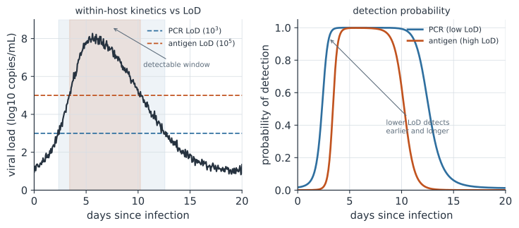
Every assay has a limit of detection (LoD): the lowest viral load it can reliably call positive. A sample is detectable only while the viral load exceeds the LoD, so the assay carves a detectable window out of the infection trajectory — the span of days during which the curve sits above the threshold. A sensitive molecular assay like RT-PCR, with an LoD around $10^3$ copies per millilitre, has a wide window that opens soon after infection and closes late. A rapid antigen test, with an LoD nearer $10^5$–$10^6$, has a narrow window clustered around the peak: it misses the early rise and the long declining tail, which is the quantitative reason antigen tests are less sensitive than PCR and why a negative antigen result early in symptoms is weak evidence.

Detection probability as a function of time#

Detection is not a hard cutoff at the LoD but a smooth transition, because of assay noise and biological variation. A convenient model makes the probability of detection a logistic function of how far the log viral load exceeds the log threshold,

$$P(\text{detect} \mid t) = \frac{1}{1 + \exp\!\big(-\beta\,[\,v(t) - \ell\,]\big)},$$

where $v(t)$ is the log viral load at time $t$, $\ell$ the log LoD, and $\beta$ the sharpness of the transition. This turns the two curves into a single interpretable object: time-varying test sensitivity. The area and position of that curve are what matter for surveillance — a lower LoD shifts the whole detection-probability curve up and out, detecting more infections and detecting them earlier (Mina et al. 2020).

The sensitivity-timeliness trade-off#

Chasing the lowest possible LoD is not always the right move. For screening to interrupt transmission, what matters is detecting people while they are still infectious, and a frequently used, fast, cheaper test with a higher LoD can outperform a sensitive but slow one, because it catches infections near the peak and returns results in time to act (Larremore et al. 2021). The detection-probability curve makes the trade-off explicit: test frequency widens the effective window by giving more chances to catch the trajectory above threshold, partly compensating for a higher LoD. The same viral-load information read in reverse turns a positive test’s quantitative signal — the PCR cycle-threshold value — into an estimate of where in the infection a person is, and even into an epidemic growth signal across a cross-section of tests (Hay et al. 2021).

A worked example#

We model a log viral-load trajectory over 20 days and compute, for a molecular assay and an antigen assay, the length of the detectable window and the peak probability of detection.

In code#

R#

day <- seq(0, 20, by = 0.1)
# Log10 viral load: rise to a peak near day 5.5, then decline.
peak_day <- 5.5
logvl <- ifelse(day <= peak_day,
                2 + (8 - 2) * (day / peak_day),
                8 - (8 - 1) * (day - peak_day) / (20 - peak_day))

detect_window <- function(log_lod) {
  above <- day[logvl >= log_lod]
  if (length(above) == 0) return(0)
  max(above) - min(above)
}
p_detect_peak <- function(log_lod, beta = 2) {
  1 / (1 + exp(-beta * (max(logvl) - log_lod)))
}

c(pcr_window_days     = detect_window(3),
  antigen_window_days = detect_window(5),
  pcr_peak_sensitivity = p_detect_peak(3),
  antigen_peak_sensitivity = p_detect_peak(5))

Python#

import numpy as np

day = np.arange(0, 20.01, 0.1)
peak_day = 5.5
# Log10 viral load: rise to a peak near day 5.5, then decline.
logvl = np.where(day <= peak_day,
                 2 + (8 - 2) * (day / peak_day),
                 8 - (8 - 1) * (day - peak_day) / (20 - peak_day))

def detect_window(log_lod):
    above = day[logvl >= log_lod]
    return 0.0 if above.size == 0 else above.max() - above.min()

def p_detect_peak(log_lod, beta=2):
    return 1 / (1 + np.exp(-beta * (logvl.max() - log_lod)))

print(f"PCR detectable window     = {detect_window(3):.1f} days")
print(f"antigen detectable window = {detect_window(5):.1f} days")
print(f"PCR peak sensitivity      = {p_detect_peak(3):.3f}")
print(f"antigen peak sensitivity  = {p_detect_peak(5):.3f}")

PCR detectable window     = 14.8 days
antigen detectable window = 8.9 days
PCR peak sensitivity      = 1.000
antigen peak sensitivity  = 0.998

Julia#

day = 0:0.1:20
peak_day = 5.5
logvl = [d <= peak_day ? 2 + (8 - 2) * (d / peak_day) :
         8 - (8 - 1) * (d - peak_day) / (20 - peak_day) for d in day]

function detect_window(log_lod)
    above = [day[i] for i in eachindex(day) if logvl[i] >= log_lod]
    isempty(above) ? 0.0 : maximum(above) - minimum(above)
end
p_detect_peak(log_lod; beta = 2) = 1 / (1 + exp(-beta * (maximum(logvl) - log_lod)))

(pcr_window = detect_window(3), antigen_window = detect_window(5),
 pcr_peak = p_detect_peak(3), antigen_peak = p_detect_peak(5))

The molecular assay’s lower threshold buys a detectable window several days wider than the antigen test’s, which is concentrated around the viral-load peak.

Why it matters#

Treating test sensitivity as a fixed number hides the fact that most false negatives are a matter of timing, not a broken test — the sample was taken while the viral load sat below the assay’s threshold. Modeling detection as the interaction of a viral-load trajectory with a limit of detection makes the diagnostic window, the sensitivity-timeliness trade-off, and the case for frequent testing quantitative rather than intuitive. It also connects the clinical and the epidemiological: the same kinetics that decide whether one test is positive decide, in aggregate, what a surveillance system can see.

Related#

• Diagnostic Testing and Screening — sensitivity, specificity, PPV, and ROC curves
• Within-Host Viral Dynamics and Infectiousness — the trajectories that set detectability
• qPCR and Rapid Antigen Tests — the assays and their limits of detection
• Surveillance Systems — what detection probability means at population scale
• Back-Calculation and Deconvolution — reading kinetics back into epidemic timing