Within-Host Viral Dynamics and Infectiousness

Between-host models like SIR treat a person as infectious for a fixed period, but inside a single host the pathogen follows a trajectory: virus grows exponentially, peaks when it runs out of cells to infect, and is then cleared. That viral-load curve is what a diagnostic test measures, what determines how infectious a person is on each day of their infection, and what antivirals try to suppress. This page builds the target-cell-limited model that produces the curve and connects its shape to the infectiousness profile that drives transmission.

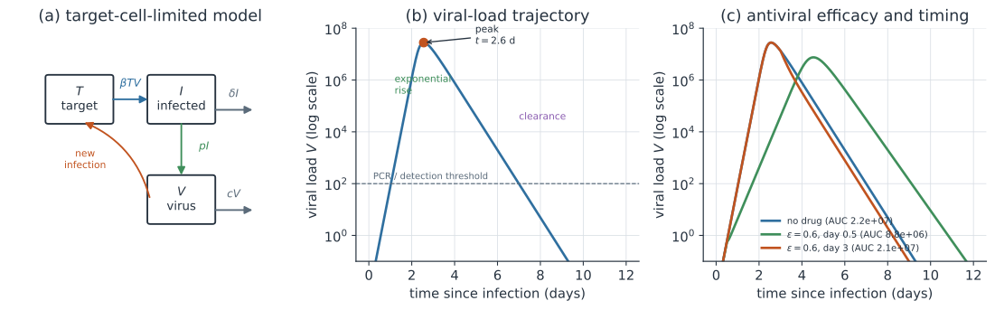
The target-cell-limited model

Track three quantities inside one host: uninfected target cells $T$ that the virus can enter, productively infected cells $I$, and free virus $V$. Virus enters target cells at rate $\beta$, infected cells die (or stop producing) at rate $\delta$ and release virus at rate $p$, and free virus is cleared at rate $c$.

$$\begin{aligned} \frac{dT}{dt} &= -\beta T V \\ \frac{dI}{dt} &= \beta T V - \delta I \\ \frac{dV}{dt} &= p I - c V \end{aligned}$$

Each rate has a direct biological reading. The term $\beta T V$ is mass-action infection of susceptible cells by circulating virus, exactly the within-host analogue of $\beta S I / N$ between hosts. The rate $\delta$ combines the intrinsic death of infected cells with immune killing, and $c$ folds antibody neutralization and physical clearance into one loss rate for virus. This lumped treatment is deliberate: the companion within-host page resolves the immune response into explicit B-cell and T-cell compartments, whereas here clearance is bundled into $\delta$ and $c$ so the focus stays on the viral-load trajectory and its epidemiological consequences. Target cells here are not replenished, which is what makes the model target-cell-limited and gives the viral load a single peak rather than a persistent set point.

Within-host $R_0$ and the invasion condition

Early in infection, target cells are still near their starting level $T_0$, so the equations for $I$ and $V$ are approximately linear. One infected cell survives for a mean time $1/\delta$ and sheds virus at rate $p$, producing $p/\delta$ virions; each virion survives $1/c$ and infects target cells at rate $\beta T_0$, producing $\beta T_0/c$ newly infected cells. Multiplying the two chains gives the within-host basic reproduction number.

$$R_0^{\text{wh}} = \frac{\beta T_0 p}{\delta c}$$

Infection takes off only when $R_0^{\text{wh}} > 1$; otherwise the inoculum clears before it can establish. When it does exceed one, the viral load grows exponentially at a rate set by the same parameters, so a larger $R_0^{\text{wh}}$ means both a higher chance of establishment and a faster climb to peak.

The viral-load trajectory and infectiousness

The trajectory has three phases, visible in panel (b). Virus first grows exponentially while target cells are abundant, then the growing infected-cell population depletes target cells, and once too few remain to sustain replication the load reaches a peak. After the peak, production falls behind clearance and the viral load declines toward extinction, at a rate governed by $\delta$ and $c$. The height of the peak is set mainly by the size of the initial susceptible-cell pool, because that is the fuel the epidemic-in-miniature consumes.

This curve is the bridge to transmission. A person’s infectiousness on a given day rises and falls roughly with their viral load, often through a saturating relationship, so the shedding profile inherits the shape of $V(t)$: low early, highest around the peak, then tapering. That time-varying infectiousness is exactly the generation-interval distribution used at the population scale, so the within-host peak timing helps explain why the generation and serial intervals have the means and shapes they do, and it feeds the renewal-equation link between growth rate and reproduction number developed on the Euler–Lotka page. The gap between the moment the load crosses the transmission threshold and the moment symptoms appear is what creates a pre-symptomatic infectious window when the viral peak precedes symptom onset.

Detection follows the same curve. A PCR assay reports a positive result once the viral load rises above its limit of detection, and the cycle-threshold (Ct) value is inversely related to load, so Ct falls to a minimum near the peak and rises again during clearance. The dashed line in panel (b) marks such a threshold: it defines the latent period before a test can catch the infection, the window of test positivity, and the tail during which residual RNA keeps a test positive after the person is no longer infectious. Modelling within-host dynamics ties together the mechanistic paths from infection to shedding, symptoms, and a positive test, the multi-scale view developed in the nested within–between-host models page and put to work by Perelson (2002).

Antiviral effects

An antiviral can be represented as reducing one of the rates by an efficacy $\varepsilon \in [0, 1]$. A drug that blocks cell entry lowers $\beta$ to $(1-\varepsilon)\beta$, while one that blocks replication or assembly lowers production $p$ to $(1-\varepsilon)p$; either lowers $R_0^{\text{wh}}$ by the factor $(1-\varepsilon)$. If the treated $R_0^{\text{wh}}$ drops below one the infection is aborted, but even a partial reduction blunts and delays the peak and shrinks the area under the viral-load curve, the within-host analogue of drug exposure in the pharmacodynamics story. Timing is as important as efficacy: panel (c) shows that starting the same drug early flattens the peak and cuts the area under the curve sharply, whereas starting after the peak has largely formed removes only the tail. This is why antivirals such as oseltamivir for influenza or nirmatrelvir for SARS-CoV-2 are most effective when given in the first days of symptoms, before the viral load has already crested.

A worked example

Take scaled parameters $\beta = 5\times10^{-7}$, $\delta = 3$ per day, $p = 40$ per day, $c = 6$ per day, with $T_0 = 10^{7}$ target cells. The within-host reproduction number is $$R_0^{\text{wh}} = \frac{\beta T_0 p}{\delta c} = \frac{5\times10^{-7}\cdot 10^{7}\cdot 40}{3 \cdot 6} \approx 11,$$ so the infection establishes readily and the viral load climbs to a peak near $2.8\times10^{7}$ around day 2.6 before clearing. A drug that cuts production $p$ by 60% starting on day 0.5 keeps the treated reproduction number above one, so infection still occurs, but the peak load falls by roughly a factor of four.

In code

We integrate the target-cell-limited model, print the within-host $R_0$ and the peak viral load, then repeat with a drug that reduces production $p$ and print the reduced peak. The system is stiff, so we use an implicit solver.

R

library(deSolve)

pars <- c(beta = 5e-7, delta = 3, p = 40, c = 6)
T0 <- 1e7

tcl <- function(t, y, pr, eps = 0, t_treat = 0) {
  with(as.list(c(y, pr)), {
    p_eff <- if (t >= t_treat) p * (1 - eps) else p
    list(c(dT = -beta * T * V,
           dI = beta * T * V - delta * I,
           dV = p_eff * I - c * V))
  })
}

y0 <- c(T = T0, I = 0, V = 1e-2)
tt <- seq(0, 12, by = 0.01)
R0 <- with(as.list(pars), beta * T0 * p / (delta * c))

untreated <- ode(y0, tt, tcl, pars)
treated   <- ode(y0, tt, tcl, pars, eps = 0.6, t_treat = 0.5)
c(R0 = R0,
  peak_untreated = max(untreated[, "V"]),
  peak_treated   = max(treated[, "V"]))

Python

import numpy as np
from scipy.integrate import solve_ivp

beta, delta, p, c = 5e-7, 3.0, 40.0, 6.0
T0, V0 = 1e7, 1e-2
R0 = beta * T0 * p / (delta * c)


def peak_load(eps=0.0, t_treat=0.0):
    def rhs(t, y):
        T, I, V = y
        p_eff = p * (1 - eps) if t >= t_treat else p
        return [-beta * T * V, beta * T * V - delta * I, p_eff * I - c * V]
    sol = solve_ivp(rhs, [0, 12], [T0, 0.0, V0], method="LSODA",
                    rtol=1e-9, atol=1e-9, dense_output=True)
    t = np.linspace(0, 12, 3000)
    return sol.sol(t)[2].max()


print(f"within-host R0 = {R0:.1f}")
print(f"untreated peak viral load = {peak_load():.2e}")
print(f"treated peak (60% drop in p from day 0.5) = {peak_load(0.6, 0.5):.2e}")

within-host R0 = 11.1
untreated peak viral load = 2.79e+07
treated peak (60% drop in p from day 0.5) = 7.52e+06

Julia

using DifferentialEquations

function tcl!(du, y, pr, t)
    T, I, V = y
    beta, delta, p, c, eps, t_treat = pr
    p_eff = t >= t_treat ? p * (1 - eps) : p
    du[1] = -beta * T * V
    du[2] = beta * T * V - delta * I
    du[3] = p_eff * I - c * V
end

y0 = [1e7, 0.0, 1e-2]
untreated = solve(ODEProblem(tcl!, y0, (0.0, 12.0),
    (5e-7, 3.0, 40.0, 6.0, 0.0, 0.0)), Rosenbrock23())
treated = solve(ODEProblem(tcl!, y0, (0.0, 12.0),
    (5e-7, 3.0, 40.0, 6.0, 0.6, 0.5)), Rosenbrock23())
maximum(u[3] for u in untreated.u)   # untreated peak viral load

Why it matters

The viral-load trajectory is the hinge between two scales. Downward, it links the molecular events of replication and clearance to what a diagnostic test reports and when. Upward, it sets the day-by-day infectiousness that becomes the generation interval, so the timing of the within-host peak helps decide whether an epidemic can be outrun by symptom-based control. The same curve grounds the trade-offs in the evolution of virulence: a virus that replicates faster reaches a higher transmissible peak but may deplete target cells and provoke clearance sooner, the between-host cost-benefit written one scale down.

Related

• Pharmacodynamics
• Within-Host Dynamics and the Immune Response
• Adaptive Dynamics and the Evolution of Virulence
• The Euler–Lotka Equation
• Epidemiological Intervals and Delays
• Multi-Scale (Nested) Models
• Epidemiology