The Euler–Lotka Equation: From Growth Rate to R₀

Early in an outbreak the one thing you can measure cleanly is the growth rate: cases are doubling every few days. What you actually want is the reproduction number, because that is what tells you how hard the epidemic is to stop. The Euler–Lotka (renewal) equation is the exact bridge between the two, and it carries a surprise: the same growth rate implies a different $R_0$ depending on the shape of the generation interval.

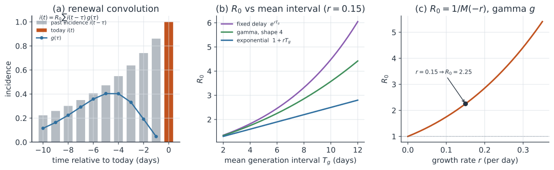
The renewal equation

Write $i(t)$ for the number of new infections at time $t$ and $g(\tau)$ for the generation-interval distribution, the normalized probability that transmission from an infected person happens a time $\tau$ after their own infection. Each person infected at time $t-\tau$ contributes, on average, $R_0\,g(\tau)$ new infections a time $\tau$ later. Summing over all past infection times gives the renewal equation:

$$i(t) = R_0 \int_0^\infty i(t-\tau)\, g(\tau)\, \mathrm{d}\tau .$$

Today’s incidence is a convolution of past incidence with the infectiousness profile, scaled by $R_0$. This is the continuous-time parent of the discrete renewal equation used to estimate the effective reproduction number, and it is the same accounting that a branching process does one generation at a time.

From $r$ to $R_0$

During the early phase incidence grows exponentially, $i(t) \propto e^{rt}$, where $r$ is the growth rate. Substitute $i(t) = i_0 e^{rt}$ into the renewal equation:

$$i_0 e^{rt} = R_0 \int_0^\infty i_0 e^{r(t-\tau)}\, g(\tau)\, \mathrm{d}\tau = R_0\, e^{rt} \int_0^\infty e^{-r\tau}\, g(\tau)\, \mathrm{d}\tau .$$

The $e^{rt}$ cancels, leaving the Euler–Lotka equation:

$$\frac{1}{R_0} = \int_0^\infty e^{-r\tau}\, g(\tau)\, \mathrm{d}\tau = M(-r),$$

where $M(s) = \mathbb{E}[e^{s\tau}]$ is the moment-generating function of the generation interval. So $R_0 = 1/M(-r)$: read off the growth rate, know the generation-interval distribution, and $R_0$ follows exactly.

This is the epidemiological twin of the demographic Euler–Lotka equation for an age-structured population,

$$\int_0^\infty e^{-r a}\, \ell_a\, m_a\, \mathrm{d}a = 1,$$

where $\ell_a$ is survival to age $a$ and $m_a$ is fecundity at age $a$ (the machinery behind reproductive value). An infection’s generation interval plays the role of a mother’s age-specific reproduction, and $R_0$ is the net reproduction number.

Why the shape of the generation interval matters

The map $R_0 = 1/M(-r)$ depends on the whole distribution $g$, not just its mean. Three tractable cases make the point, all with the same mean generation interval $T_g$ and the same growth rate $r$.

Fixed delay. If everyone transmits exactly $T_g$ after infection, $g$ is a spike at $T_g$ and $M(-r) = e^{-rT_g}$, so

$$R_0 = e^{r T_g}.$$

This is the largest $R_0$ any distribution with mean $T_g$ can give.

Exponential interval. If $g$ is exponential with mean $T_g$, then $M(-r) = 1/(1 + r T_g)$ and

$$R_0 = 1 + r T_g,$$

the familiar linear approximation, and the smallest $R_0$ in the gamma family.

Gamma interval. A gamma generation interval with mean $T_g$ and shape $a$ (so scale $T_g/a$) gives

$$R_0 = \left(1 + \frac{r T_g}{a}\right)^{a},$$

which interpolates between the two: $a=1$ is exponential, and $a\to\infty$ recovers the fixed-delay $e^{r T_g}$.

Two lessons follow. For a fixed $r$, a longer mean generation interval implies a larger $R_0$, because the same growth has to be packed into slower cycles. For a fixed mean, less variable intervals (larger shape $a$) imply a larger $R_0$, because concentrating transmission in time makes a given growth rate demand more secondary cases per generation. Assuming an exponential interval when the truth is nearly fixed can badly understate $R_0$.

Practical caution

Two cautions matter in practice.

First, we almost never observe the generation interval directly, because the moment of infection is unseen; the serial interval (onset to onset) is the usual proxy. The serial interval has the same mean as the generation interval under simple assumptions but a larger variance, so plugging it into Euler–Lotka as if it were $g$ biases $R_0$.

Second, mis-specifying $g$ propagates straight into $R_0$. Wallinga & Lipsitch showed that the relationship between $r$ and $R_0$ is governed entirely by the generation-interval distribution, and that different plausible distributions consistent with the same data can yield materially different $R_0$ (Wallinga & Lipsitch 2007, doi:10.1098/rspb.2006.3754). Park et al. developed a practical generation-interval-based approach that makes these dependencies explicit and quantifies how uncertainty in $g$ maps to uncertainty in the inferred strength of an epidemic (Park et al. 2019, doi:10.1016/j.epidem.2018.12.002).

A worked example

Take a gamma generation interval with mean $T_g = 6$ days and shape $a = 4$, and an observed growth rate $r = 0.15$ per day (roughly a 4.6-day doubling time). The Euler–Lotka answer is

$$R_0 = \left(1 + \frac{0.15 \times 6}{4}\right)^{4} = (1.225)^{4} \approx 2.25 .$$

The exponential-interval approximation for the same mean would give $R_0 = 1 + 0.15\times 6 = 1.9$, and the fixed-delay extreme would give $R_0 = e^{0.15\times 6} = e^{0.9} \approx 2.46$. The same growth rate spans $R_0$ from $1.9$ to $2.46$ purely through the assumed interval shape.

In code

We compute $R_0$ from $r$ via $1/M(-r)$, then simulate the renewal equation forward at that $R_0$ and recover the growth rate as a round-trip check.

R

r <- 0.15; shape <- 4; mean_gi <- 6; scale <- mean_gi / shape

# Continuous Euler-Lotka: R0 = 1 / M(-r), M(-r) = (1 + r*scale)^(-shape)
R0_mgf <- (1 + r * scale)^shape

# Discretized generation interval on days 1..40
tau <- 1:40
g <- dgamma(tau, shape = shape, scale = scale); g <- g / sum(g)
R0_disc <- 1 / sum(exp(-r * tau) * g)             # discrete Euler-Lotka

# Round-trip: seed the renewal recursion, recover the growth rate
T <- 160; inc <- numeric(T); inc[1] <- 1
for (t in 2:T) {
  s <- 1:min(t - 1, length(g))
  inc[t] <- R0_disc * sum(inc[t - s] * g[s])
}
r_hat <- coef(lm(log(inc[90:140]) ~ I(90:140)))[2]
c(R0_mgf = R0_mgf, R0_disc = R0_disc, r_hat = r_hat)

Python

We use SciPy for the gamma density and NumPy for the renewal recursion.

import numpy as np
from scipy.stats import gamma as gamma_dist

r, shape, mean_gi = 0.15, 4.0, 6.0
scale = mean_gi / shape

# Continuous Euler-Lotka: R0 = 1 / M(-r), M(-r) = (1 + r*scale)^(-shape)
R0_mgf = (1 + r * scale) ** shape
print(f"R0 (continuous MGF)  = {R0_mgf:.3f}")

# Discretized generation interval on days 1..40
tau = np.arange(1, 41)
g = gamma_dist.pdf(tau, a=shape, scale=scale)
g = g / g.sum()
R0_disc = 1.0 / np.sum(np.exp(-r * tau) * g)      # discrete Euler-Lotka
print(f"R0 (discrete kernel) = {R0_disc:.3f}")

# Round-trip: seed the renewal recursion, recover the realized growth rate
T = 160
inc = np.zeros(T); inc[0] = 1.0
for t in range(1, T):
    s = np.arange(1, min(t, len(g)) + 1)
    inc[t] = R0_disc * np.sum(inc[t - s] * g[s - 1])
win = np.arange(90, 140)
r_hat = np.polyfit(win, np.log(inc[win]), 1)[0]
print(f"target r = {r:.3f}, realized r = {r_hat:.3f}")

R0 (continuous MGF)  = 2.252
R0 (discrete kernel) = 2.251
target r = 0.150, realized r = 0.150

The realized growth rate returns the value we started from, confirming that $R_0 = 1/M(-r)$ and the renewal equation are two views of the same relationship.

Julia

using Distributions, Statistics

r, shape, mean_gi = 0.15, 4.0, 6.0
scale = mean_gi / shape

R0_mgf = (1 + r * scale)^shape                    # continuous Euler-Lotka

tau = 1:40
g = pdf.(Gamma(shape, scale), tau); g ./= sum(g)
R0_disc = 1 / sum(exp.(-r .* tau) .* g)           # discrete Euler-Lotka

T = 160; inc = zeros(T); inc[1] = 1.0
for t in 2:T
    s = 1:min(t - 1, length(g))
    inc[t] = R0_disc * sum(inc[t .- s] .* g[s])
end
X = hcat(ones(51), 90:140)
r_hat = (X \ log.(inc[90:140]))[2]
(R0_mgf = R0_mgf, R0_disc = R0_disc, r_hat = r_hat)

Why it matters

The Euler–Lotka equation is why a growth rate alone is never enough to name a reproduction number. Report a doubling time and you have pinned $r$, but $R_0$ still depends on the generation interval you assume, and the gap between plausible assumptions can be the difference between “hard to stop” and “very hard to stop.” This is the exact link that turns the messy, early-outbreak signal we can see (speed) into the control-relevant quantity we care about (strength), and it is why estimating the generation interval well is inseparable from estimating $R_0$.

Related

• Epidemiological Intervals and Delays
• The Next-Generation Matrix and R₀
• The Effective Reproduction Number and Forecasting
• The Renewal Equation
• Moment Generating Functions
• Reproductive Value
• Branching Processes
• Epidemiology