Reproductive Value and Demographic Sensitivity

A newborn and a prime-aged adult do not count equally toward a population’s future: the adult has already survived the risky early stages and is reproducing now, while the newborn still has to run that gauntlet. Reproductive value makes this precise as the expected future reproductive contribution of an individual conditional on its current age or stage, and it turns out to be the left eigenvector of the projection matrix. That same vector, paired with the stable stage distribution, tells you exactly where a change in a vital rate moves the growth rate most — the practical payoff for targeting selection or control.

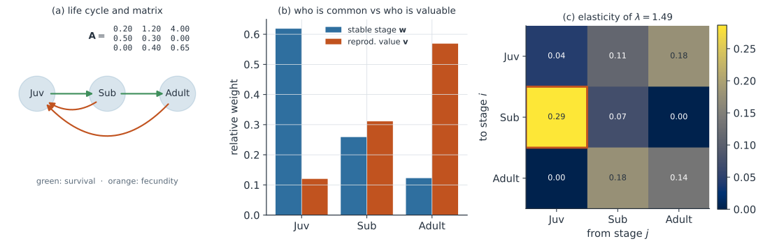
Reproductive value for a three-stage life cycle: the life-cycle graph and its matrix, the stable stage distribution versus reproductive value, and the elasticity of the growth rate to each transition.

Two eigenvectors of the projection matrix

A structured population model projects a stage vector forward with $\mathbf{n}_{t+1}=\mathbf{A}\,\mathbf{n}_t$ , and its long-run behavior is set by the eigenvalues and eigenvectors of $\mathbf{A}$ . The dominant eigenvalue $\lambda$ is the asymptotic growth rate, and it comes with two eigenvectors that read very differently.

The right eigenvector $\mathbf{w}$ solves $\mathbf{A}\mathbf{w}=\lambda\mathbf{w}$ and gives the stable stage distribution — the proportions in each class once transients decay. The left eigenvector $\mathbf{v}$ solves $\mathbf{v}^\top\mathbf{A}=\lambda\mathbf{v}^\top$ and gives reproductive value — the relative expected contribution of each class to the distant future. Entry $v_i$ answers a targeting question: if you could add one individual to the population, how much would seeding it into class $i$ raise long-run numbers.

These two vectors are the projection’s answer to “who is common” ( $\mathbf{w}$ ) versus “who is valuable” ( $\mathbf{v}$ ), and they are generally not proportional. Newborns dominate $\mathbf{w}$ because most individuals are young, yet reproducing adults dominate $\mathbf{v}$ because they are the ones about to produce offspring. Reproductive value is also the weighting that makes total population size grow smoothly: the scalar $V_t=\mathbf{v}^\top\mathbf{n}_t$ grows by exactly $\lambda$ every step with no transient wobble, so $\mathbf{v}$ is the linearizing coordinate for a structured population.

Fisher’s discounted future offspring

R. A. Fisher introduced reproductive value in The Genetical Theory of Natural Selection (Fisher 1930) as the expected future offspring of an individual, discounted because a birth today competes against a growing population tomorrow. For an age-structured model with survivorship $\ell_x$ (probability of reaching age $x$ ) and fecundity $m_x$ , the reproductive value of an age- $a$ individual is

$v_a \;\propto\; \frac{1}{\ell_a}\sum_{x\ge a}\lambda^{-(x-a)}\,\ell_x\,m_x .$

Each future birth at age $x$ is weighted by $\ell_x/\ell_a$ , the chance of surviving from $a$ to $x$ , and discounted by $\lambda^{-(x-a)}$ because offspring born later are a smaller share of a population that has grown in the meantime. Reproductive value therefore rises through the juvenile stages as survival to reproduction becomes more assured, peaks near the onset of reproduction, and falls off in old age as the remaining reproductive future shrinks. Grafen (2006) doi:10.1007/s00285-006-0376-4 gives a formal account of why this quantity is the correct maximand for natural selection in an age-structured population.

Sensitivity and elasticity

Reproductive value earns its keep through sensitivity analysis (Caswell 2001; Caswell 2010 doi:10.4054/DemRes.2010.23.19). The sensitivity of the growth rate to a change in matrix entry $a_{ij}$ is the outer product of reproductive value and the stable stage distribution,

$\frac{\partial\lambda}{\partial a_{ij}} \;=\; \frac{v_i\,w_j}{\mathbf{v}^\top\mathbf{w}} .$

The reading is direct: a perturbation to the $j\to i$ transition matters in proportion to how many individuals are in the source class $j$ (given by $w_j$ ) times how valuable the destination class $i$ is (given by $v_i$ ). Elasticities are the proportional version, $e_{ij}=(a_{ij}/\lambda)\,\partial\lambda/\partial a_{ij}$ , and they have the convenient property of summing to one, so they partition the growth rate among life-cycle transitions and rank them on a common scale. The transition with the largest elasticity is where a proportional intervention on a vital rate — a management action, a control effort, a selective pressure — buys the most change in $\lambda$ .

A worked example

Take a three-stage Lefkovitch matrix for juveniles, subadults, and adults,

$\mathbf{A}=\begin{pmatrix} 0.20 & 1.20 & 4.00 \\ 0.50 & 0.30 & 0.00 \\ 0.00 & 0.40 & 0.65 \end{pmatrix},$

where the top row is fecundity, the sub-diagonal is survival-and-advance, and the diagonal holds individuals that survive but stay in their stage. The dominant eigenvalue is $\lambda\approx 1.495$ , so the population grows about $50\%$ per step. The stable stage distribution is $\mathbf{w}\approx(0.619,\,0.259,\,0.123)$ : most individuals are juveniles. Reproductive value, scaled so a juvenile is $1$ , is $\mathbf{v}\approx(1,\,2.59,\,4.73)$ : an adult is worth nearly five juveniles for the population’s future. The elasticities sum to one, and the largest belongs to the juvenile-to-subadult survival transition at $0.287$ — small improvements there move growth more than anything else in the life cycle.

In code

We build $\mathbf{A}$ , extract $\lambda$ , $\mathbf{w}$ , and $\mathbf{v}$ , form the sensitivity matrix $\mathbf{v}\mathbf{w}^\top/(\mathbf{v}^\top\mathbf{w})$ , and report the top-elasticity transition.

R

library(popbio)

A <- matrix(c(0.20, 1.20, 4.00,
              0.50, 0.30, 0.00,
              0.00, 0.40, 0.65), nrow = 3, byrow = TRUE)

ea <- eigen.analysis(A)          # popbio does the whole decomposition
ea$lambda1                        # dominant eigenvalue ~1.495
$ea$stable.stage                   # right eigenvector w
$ea$repro.value                    # left eigenvector v (reproductive value)
$ea$elasticities                   # elasticities, summing to 1
$```

### Python

```python
import numpy as np

# Stage matrix: juvenile, subadult, adult (rows = to, cols = from).
A = np.array([[0.20, 1.20, 4.00],
              [0.50, 0.30, 0.00],
              [0.00, 0.40, 0.65]])
stages = ["Juv", "Sub", "Adult"]

vals, vecs = np.linalg.eig(A)
i = int(np.argmax(vals.real))
lam = vals[i].real
w = np.abs(vecs[:, i].real); w /= w.sum()        # stable stage (right)
lv, lvec = np.linalg.eig(A.T)
j = int(np.argmax(lv.real))
v = np.abs(lvec[:, j].real); v /= v[0]            # reproductive value (left)

sens = np.outer(v, w) / (v @ w)                   # sensitivity of lambda
elas = (A / lam) * sens                           # elasticity (sums to 1)
r, c = np.unravel_index(np.argmax(elas), elas.shape)

print(f"lambda = {lam:.3f}")
print(f"stable stage w = {np.round(w, 3)}")
print(f"reproductive value v = {np.round(v, 2)} (juvenile = 1)")
print(f"elasticities sum to {elas.sum():.3f}")
print(f"top transition: {stages[c]} -> {stages[r]} (elasticity {elas[r, c]:.3f})")

lambda = 1.495
stable stage w = [0.619 0.259 0.123]
reproductive value v = [1.   2.59 4.73] (juvenile = 1)
elasticities sum to 1.000
top transition: Juv -> Sub (elasticity 0.287)

Julia

using LinearAlgebra

A = [0.20 1.20 4.00;
     0.50 0.30 0.00;
     0.00 0.40 0.65]

vals, vecs = eigen(A)
i = argmax(real.(vals)); lam = real(vals[i])
w = abs.(real.(vecs[:, i])); w ./= sum(w)          # stable stage
lv, lvec = eigen(permutedims(A))
j = argmax(real.(lv))
v = abs.(real.(lvec[:, j])); v ./= v[1]             # reproductive value

sens = (v * w') ./ dot(v, w)                        # sensitivity matrix
elas = (A ./ lam) .* sens                           # elasticities
lam, w, v

Why it matters

Reproductive value is the right currency for targeting, and in disease ecology the “individuals” are host classes. When hosts differ by age, stage, or spatial patch, some classes contribute far more to future transmission than a headcount suggests, and reproductive value from the transmission-projection operator quantifies exactly that contribution. The next-generation matrix is the epidemiological analogue of the projection matrix, and its left eigenvector plays the reproductive-value role: it tells you which infected class seeds the most future infections, so control aimed there moves $R_0$ most per unit effort. The same sensitivity logic that ranks life-cycle transitions for a manager ranks transmission routes for an epidemiologist, which is why value-weighting recurs across life-history theory, source–sink dynamics, and the Euler–Lotka accounting of generations.