Force of Infection and Serocatalytic Models

The force of infection is the rate at which susceptible people become infected — the hazard of infection per unit time. It is the single quantity that connects a transmission model to the serological data we can actually collect, because the older a population is, the longer it has been exposed to that hazard, and the more of it has been infected. Reading the force of infection off an age-stratified serosurvey is one of the oldest and most useful tricks in infectious disease epidemiology.

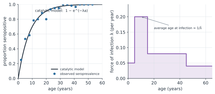
The catalytic model#

Treat the force of infection $\lambda$ as a constant hazard, the same idea as a constant hazard in survival analysis. A person of age $a$ has been exposed to that hazard for $a$ years, so the probability they have been infected at least once — and, for a lasting-immunity marker, are now seropositive — is

$$P(\text{seropositive} \mid a) = 1 - e^{-\lambda a}.$$

This is the catalytic model, introduced by Muench in the 1930s by analogy with a chemical reaction proceeding at a constant rate. Seroprevalence rises with age toward one, steeply when $\lambda$ is large and gently when it is small, and fitting that rise to survey data recovers $\lambda$. The name serocatalytic is used when the marker is a serological antibody, which is the usual case.

Age-varying force of infection#

A constant hazard is often too simple. Contact rates differ sharply by age, so children in school experience a much higher force of infection than adults, and the seroprevalence curve bends accordingly. The catalytic model generalizes by letting the hazard vary with age, $\lambda(a)$, so that

$$P(\text{seropositive} \mid a) = 1 - \exp\!\left(-\int_0^a \lambda(u)\, du\right),$$

with the integral being the cumulative hazard by age $a$. Fitting a piecewise-constant $\lambda(a)$ across age bands, as in the right panel of the figure, reveals the age structure of transmission — typically a peak in school-age children — which is exactly the pattern that a social contact matrix predicts.

Average age at infection and R₀#

The force of infection carries two further quantities. The average age at infection for a constant hazard is

$$A = \frac{1}{\lambda},$$

so a high force of infection means people are infected young. For an endemic, immunizing infection in a population with life expectancy $L$, the basic reproduction number is approximately

$$R_0 \approx 1 + \frac{L}{A} = 1 + L\lambda,$$

which lets a serosurvey — through nothing more than the age pattern of antibodies — produce an estimate of $R_0$. This relationship is why childhood infections with a young average age at infection, like measles before vaccination, have such high reproduction numbers.

A worked example#

We take age-stratified serosurvey counts generated with a true force of infection, fit the constant-hazard catalytic model by maximum likelihood, and recover the average age at infection and an estimate of $R_0$.

In code#

R#

set.seed(1834)
lam_true <- 0.12; L <- 70
ages <- 1:60
n <- rep(50, length(ages))
pos <- rbinom(length(ages), n, 1 - exp(-lam_true * ages))

# Maximum-likelihood fit of the constant-hazard catalytic model.
negll <- function(lam) -sum(dbinom(pos, n, 1 - exp(-lam * ages), log = TRUE))
lam_hat <- optimize(negll, interval = c(1e-4, 1))$minimum

A <- 1 / lam_hat
R0 <- 1 + L / A
round(c(lambda = lam_hat, avg_age = A, R0 = R0), 3)

Python#

import numpy as np
from scipy import stats
from scipy.optimize import minimize_scalar

rng = np.random.default_rng(1834)
lam_true, L = 0.12, 70
ages = np.arange(1, 61)
n = np.full(ages.size, 50)
pos = rng.binomial(n, 1 - np.exp(-lam_true * ages))

# Maximum-likelihood fit of the constant-hazard catalytic model.
def negll(lam):
    return -stats.binom.logpmf(pos, n, 1 - np.exp(-lam * ages)).sum()

lam_hat = minimize_scalar(negll, bounds=(1e-4, 1), method="bounded").x
A = 1 / lam_hat
R0 = 1 + L / A

print(f"force of infection lambda = {lam_hat:.3f} per year")
print(f"average age at infection  = {A:.1f} years")
print(f"implied R0                = {R0:.2f}")

force of infection lambda = 0.124 per year
average age at infection  = 8.1 years
implied R0                = 9.69

Julia#

using Distributions, Optim, Random

Random.seed!(1834)
lam_true, L = 0.12, 70
ages = 1:60
n = fill(50, length(ages))
pos = [rand(Binomial(n[i], 1 - exp(-lam_true * ages[i]))) for i in eachindex(ages)]

negll(lam) = -sum(logpdf(Binomial(n[i], 1 - exp(-lam * ages[i])), pos[i])
                  for i in eachindex(ages))
lam_hat = optimize(l -> negll(l[1]), [0.1], LBFGS()).minimizer[1]

A = 1 / lam_hat
R0 = 1 + L / A
(lambda = lam_hat, avg_age = A, R0 = R0)

Why it matters#

The force of infection is the bridge between serology and transmission: it turns a single cross-sectional serosurvey, which is far cheaper than following an epidemic in real time, into estimates of who is being infected, how young, and how transmissible the pathogen is. It is also the quantity that severity and burden estimates need, because the infection attack rate from a serosurvey is exactly the cumulative effect of the force of infection. When contact patterns make transmission age-specific, the serocatalytic model reads that structure straight from the shape of the seroprevalence curve.

Related#

• Social Contact Matrices and Age-Structured Mixing — the mixing that shapes the age pattern of the hazard
• Survival Analysis — hazards and cumulative hazards, the same mathematics
• Severity: Estimating the CFR and IFR — using the infection attack rate a serosurvey provides
• The Next-Generation Matrix and R₀ — R₀ in age-structured populations
• Genomic Surveillance — a complementary window on who infects whom