Pooled Testing and Prevalence Estimation

Testing specimens one at a time is wasteful when infection is rare and specimens are many. Pooled testing — combining several specimens and testing the group as one — is the efficient alternative, and it is the norm in arbovirus surveillance, where thousands of mosquitoes are trapped each week and tested in pools by species, site, and date. A positive pool means at least one infected specimen, so recovering the per-specimen prevalence from pool results takes a little modeling — and the standard quick estimate, the minimum infection rate, gets it wrong.

Why pool#

Pooling is efficient because at low prevalence most pools are negative, and one negative test clears many specimens at once — the logic Dorfman introduced for screening army recruits. For vector surveillance there is a second reason: the sheer volume. Testing tens of thousands of individual mosquitoes is infeasible, so specimens are batched into pools of a fixed maximum size (often 25 to 50), and the pool is the unit of testing. The price is that a positive pool no longer tells you how many of its specimens were infected, only that at least one was, and that is the gap the estimators below fill.

The minimum infection rate and its bias#

The minimum infection rate (MIR) is the traditional summary: the number of positive pools per thousand specimens tested,

$$\mathrm{MIR} = \frac{\text{positive pools}}{\text{total specimens}} \times 1000.$$

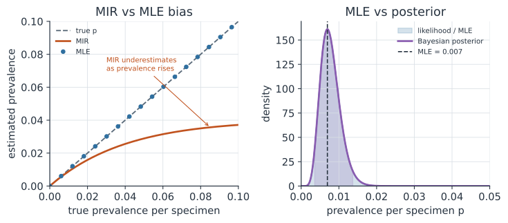
It is called minimum because it assumes each positive pool contains exactly one infected specimen — the fewest that could explain a positive. That assumption is fine when infection is rare, but as prevalence rises the chance of two or more infected specimens in a pool grows, those extra infections go uncounted, and the MIR increasingly underestimates the true prevalence. The left panel of the figure shows the bias widening with prevalence; the MIR also depends on pool size, so it is not comparable across surveillance programs that pool differently (Gu, Lampman, and Novak documented these problems for mosquito surveillance).

The maximum-likelihood estimator#

The fix is to model how pools become positive. If per-specimen prevalence is $p$ and infection is independent across specimens, a pool of size $m$ tests positive with probability

$$P(\text{pool}^+) = 1 - (1 - p)^m.$$

With $k$ positive pools out of $n$ pools of equal size $m$, the likelihood is binomial in the pools, and maximizing it gives a closed form,

$$\hat{p} = 1 - \left(1 - \frac{k}{n}\right)^{1/m}.$$

This maximum-likelihood estimate accounts for multiple infections per pool, so it is unbiased (tracking the identity line in the figure), it comes with a confidence interval, and unlike the MIR it is comparable across pool sizes (Walter, Hildreth, and Beaty 1980 gave the estimator for pools of variable size). When pools have variable sizes $m_i$ — the usual case, since the last pool of a batch is rarely full — there is no closed form, but the likelihood

$$L(p) = \prod_{i:\, \text{pool}^+} \big[1 - (1-p)^{m_i}\big] \prod_{i:\, \text{pool}^-} (1-p)^{m_i}$$

is maximized numerically, which is what tools like PooledInfRate do.

A Bayesian alternative#

The same pooled likelihood takes a Bayesian prior naturally, which is useful when counts are small — a single week’s trapping at one site — and a maximum-likelihood interval would be unstable or run to the boundary at zero positives. Placing a $\text{Beta}(a, b)$ prior on $p$ and combining it with the pooled likelihood gives a posterior that is summarized by its mean and a credible interval, and a weak prior like $\text{Beta}(1,1)$ leaves the answer close to the MLE while still returning a sensible interval when no pool is positive. The right panel shows the MLE and the uniform-prior posterior almost on top of each other for a dataset with several positives; they diverge only when the data are sparse and the prior does real work.

A worked example#

Take $n = 50$ pools of size $m = 25$, of which $k = 8$ test positive. We compute the MIR, the maximum-likelihood prevalence with a confidence interval, and the Bayesian posterior.

In code#

R#

n <- 50; m <- 25; k <- 8            # pools, pool size, positive pools

mir <- k / (n * m)                  # per specimen (multiply by 1000 to report)
p_hat <- 1 - (1 - k / n)^(1 / m)    # maximum-likelihood estimate

# Wald confidence interval via the delta method on the pool positivity.
theta <- k / n
var_theta <- theta * (1 - theta) / n
dp <- (1 / m) * (1 - theta)^(1 / m - 1)
se <- dp * sqrt(var_theta)
ci <- p_hat + c(-1.96, 1.96) * se

round(c(MIR = mir, MLE = p_hat, lower = ci[1], upper = ci[2]), 4)

Python#

import numpy as np

n, m, k = 50, 25, 8                 # pools, pool size, positive pools

mir = k / (n * m)                   # per specimen (x1000 to report as MIR)
p_hat = 1 - (1 - k / n) ** (1 / m)  # maximum-likelihood estimate

# Wald confidence interval via the delta method on the pool positivity.
theta = k / n
var_theta = theta * (1 - theta) / n
dp = (1 / m) * (1 - theta) ** (1 / m - 1)
se = dp * np.sqrt(var_theta)
lo, hi = p_hat - 1.96 * se, p_hat + 1.96 * se

print(f"MIR (per specimen) = {mir:.4f}  ({mir * 1000:.1f} per 1000)")
print(f"MLE prevalence     = {p_hat:.4f}")
print(f"95% CI             = ({lo:.4f}, {hi:.4f})")

MIR (per specimen) = 0.0064  (6.4 per 1000)
MLE prevalence     = 0.0069
95% CI             = (0.0021, 0.0118)

Julia#

n, m, k = 50, 25, 8                 # pools, pool size, positive pools

mir = k / (n * m)
p_hat = 1 - (1 - k / n)^(1 / m)     # maximum-likelihood estimate

theta = k / n
var_theta = theta * (1 - theta) / n
dp = (1 / m) * (1 - theta)^(1 / m - 1)
se = dp * sqrt(var_theta)
lo, hi = p_hat - 1.96 * se, p_hat + 1.96 * se

(MIR = mir, MLE = p_hat, lower = lo, upper = hi)

The Bayesian estimate in code#

The same pooled likelihood with a $\text{Beta}(1,1)$ prior, evaluated on a grid, gives the posterior mean and a 95% credible interval.

import numpy as np

n, m, k = 50, 25, 8
grid = np.linspace(1e-5, 0.05, 4000)

# Pooled log-likelihood: k positive pools, n - k negative pools of size m.
loglik = k * np.log(1 - (1 - grid) ** m) + (n - k) * m * np.log(1 - grid)
prior = np.ones_like(grid)                 # Beta(1, 1) is uniform on (0, 1)
post = np.exp(loglik - loglik.max()) * prior
post /= np.trapezoid(post, grid)           # normalize the posterior

cdf = np.cumsum(post) * (grid[1] - grid[0])
post_mean = np.trapezoid(grid * post, grid)
lo = grid[np.searchsorted(cdf, 0.025)]
hi = grid[np.searchsorted(cdf, 0.975)]

print(f"posterior mean       = {post_mean:.4f}")
print(f"95% credible interval = ({lo:.4f}, {hi:.4f})")

posterior mean       = 0.0078
95% credible interval = (0.0036, 0.0137)

The posterior mean sits a little above the maximum-likelihood estimate because the posterior is right-skewed, but the two are close and the intervals overlap heavily; the real value of the Bayesian version is the stable interval it still gives when positives are rare and the likelihood alone would run to the boundary.

Why it matters#

Infection rates from mosquito pools are a front-line risk indicator for arboviruses like West Nile and dengue, feeding directly into spraying and public warnings, so how the rate is computed is not a technicality. The minimum infection rate is quick but biased downward and not comparable across pool sizes, while the maximum-likelihood estimate is unbiased, comparable, and comes with an interval — reason enough to prefer it. The Bayesian version adds a stable interval for the sparse, zero-positive weeks that dominate off-season surveillance, and both extend cleanly to the variable pool sizes real trapping produces.

Related#

• Diagnostic Testing and Screening — sensitivity, specificity, and screening design
• Vector-Borne Disease Models — the transmission the infection rate feeds
• Maximum Likelihood Estimation — the estimator derived here
• Bayesian Inference — the prior-plus-likelihood alternative
• One Health Surveillance — vector surveillance in the wider monitoring system