Antimicrobial Resistance Across Scales

Antimicrobial resistance is hard to think about because two, often conflicting, decisions are at play with different goals acting on the same biologic process. A clinician treats a single patient and wants that infection cured, which argues for hitting the pathogen hard, balancing the other risks of antimicrobial exposure (i.e., microbiome disruption, processing of the agent by the body). The antimicrobial stewardship/ public health perspective takes the perspective of sharing a drug across a whole population and wants resistance kept rare, which argues for using any antimicrobial sparingly. The pathogen, however, does not experience these as separate problems. The drug a clinician gives to clear an infection is also the selection pressure that, summed over every prescription, decides which strains circulate next year.

This page follows that tension down through the scales. It starts with the population-level accounting of who wins the competition between sensitive and resistant strains, drops to the within-host ecology that actually generates resistant cells inside a treated patient, and then joins the two into a single nested model of malaria, following the cross-scale approach of Mideo, Alizon & Day (2008). The companion pages Population Dynamics of Resistance, The Evolution of Resistance, and Nested Within- and Between-Host Models each develop one piece in isolation; the point here is to hold them together.

The tension, stated plainly#

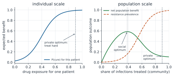
For a single patient, more drug is almost always better through the lens of resistance and clearance. Higher exposure clears the infection faster and more reliably, and clearing the sensitive population quickly also denies resistance the time it needs to arise de novo. The individual optimal choice sits at the top of the left panel above.

For the population, the same drug is a finite common resource. Every course of treatment adds a little selection pressure, and once resistance is common the drug stops working for everyone. The right panel discounts the direct benefit of treating a larger share of infections by the efficacy lost to resistance, and the net curve peaks at a moderate treatment rate. The private optimum and the social optimum do not coincide, which is the structure of a tragedy of the commons and the reason stewardship is a coordination problem rather than only a dosing problem.

The rest of the page makes each panel mechanistic.

The population scale: two strains competing for hosts#

Start with the accounting the right panel summarizes. Track the fraction of hosts that are susceptible ($S$), infected with a drug-sensitive strain ($I_s$), or infected with a resistant strain ($I_r$). The sensitive strain transmits at rate $\beta$ and is cleared naturally at rate $\gamma$ and by treatment at rate $\tau$. The resistant strain transmits at rate $\beta(1-c)$, where $c$ is the fitness cost of resistance, and treatment does nothing to it. Treated sensitive infections turn into resistant ones at a small rate $\rho\tau$, the de novo emergence that the next section derives from within-host biology.

$$\begin{aligned} \frac{dI_s}{dt} &= \beta S I_s - \gamma I_s - \tau I_s \\ \frac{dI_r}{dt} &= \beta(1-c)\, S I_r - \gamma I_r + \rho\tau I_s \\ \frac{dS}{dt} &= \gamma(I_s + I_r) + (1-\rho)\tau I_s - \beta S I_s - \beta(1-c)\, S I_r \end{aligned}$$

Each strain has an effective reproduction number at the shared susceptible level $S$. Treatment adds to clearance for the sensitive strain but leaves the resistant strain untouched:

$$R_s = \frac{\beta S}{\gamma + \tau}, \qquad R_r = \frac{\beta(1-c)\, S}{\gamma}.$$

Setting $R_s = R_r$ gives the treatment rate at which the two strains are equally fit,

$$\tau^\ast = \frac{\gamma c}{1 - c}.$$

Below $\tau^\ast$ the faster sensitive strain wins and resistance stays rare. Above $\tau^\ast$ the drug clears sensitive infections fast enough that the slower, drug-proof resistant strain takes over. A larger fitness cost $c$ pushes $\tau^\ast$ higher, so a costly resistance mutation is held in check until drug use climbs. This is the population-scale meaning of “selection”: the community treatment rate, not any one prescription, sets the direction of change.

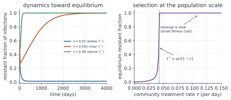
The dynamics also explain why resistance is slow to reverse. Once the resistant strain is established and the susceptible pool has shifted, cutting drug use back below $\tau^\ast$ does not restore the sensitive strain quickly, because reversal is limited by the small fitness cost acting over many transmission generations (Andersson & Levin 1999). If the cost is near zero, resistance persists almost indefinitely after the selective pressure is gone.

In code#

Integrate the two-strain model to steady state and read off the resistant fraction $I_r/(I_s+I_r)$ for a few treatment rates, then confirm the threshold $\tau^\ast$.

import numpy as np
from scipy.integrate import solve_ivp

beta, gamma, cost, rho = 0.30, 0.10, 0.30, 0.01
tau_star = gamma * cost / (1 - cost)


def rhs(t, y, tau):
    S, Is, Ir = y
    new_s = beta * S * Is
    new_r = beta * (1 - cost) * S * Ir
    dIs = new_s - gamma * Is - tau * Is
    dIr = new_r - gamma * Ir + rho * tau * Is
    dS = gamma * (Is + Ir) + (1 - rho) * tau * Is - new_s - new_r
    return [dS, dIs, dIr]


def resistant_fraction(tau):
    sol = solve_ivp(rhs, [0, 8000], [0.98, 0.01, 0.01],
                    args=(tau,), rtol=1e-9, atol=1e-11)
    S, Is, Ir = sol.y[:, -1]
    return Ir / (Is + Ir)


print(f"threshold tau* = {tau_star:.3f} per day")
for tau in (0.02, 0.045, 0.08):
    print(f"tau={tau:.3f}/day  resistant fraction={resistant_fraction(tau):.3f}")

threshold tau* = 0.043 per day
tau=0.020/day  resistant fraction=0.012
tau=0.045/day  resistant fraction=1.000
tau=0.080/day  resistant fraction=1.000

library(deSolve)

beta <- 0.30; gamma <- 0.10; cost <- 0.30; rho <- 0.01
tau_star <- gamma * cost / (1 - cost)          # exclusion threshold

rhs <- function(t, y, p) {
  S <- y[1]; Is <- y[2]; Ir <- y[3]; tau <- p$tau
  new_s <- beta * S * Is
  new_r <- beta * (1 - cost) * S * Ir
  dIs <- new_s - gamma * Is - tau * Is
  dIr <- new_r - gamma * Ir + rho * tau * Is
  dS  <- gamma * (Is + Ir) + (1 - rho) * tau * Is - new_s - new_r
  list(c(dS, dIs, dIr))
}

resistant_fraction <- function(tau) {
  out <- ode(c(0.98, 0.01, 0.01), seq(0, 8000, 10), rhs, list(tau = tau))
  last <- out[nrow(out), ]
  last[4] / (last[3] + last[4])                # Ir / (Is + Ir)
}
sapply(c(0.02, 0.045, 0.08), resistant_fraction)

using DifferentialEquations

beta, gamma, cost, rho = 0.30, 0.10, 0.30, 0.01
tau_star = gamma * cost / (1 - cost)

function rhs!(du, u, tau, t)
    S, Is, Ir = u
    new_s = beta * S * Is
    new_r = beta * (1 - cost) * S * Ir
    du[1] = gamma*(Is+Ir) + (1-rho)*tau*Is - new_s - new_r
    du[2] = new_s - gamma*Is - tau*Is
    du[3] = new_r - gamma*Ir + rho*tau*Is
end

function resistant_fraction(tau)
    prob = ODEProblem(rhs!, [0.98, 0.01, 0.01], (0.0, 8000.0), tau)
    u = solve(prob, Tsit5(); reltol = 1e-9).u[end]
    u[3] / (u[2] + u[3])
end
resistant_fraction.((0.02, 0.045, 0.08))

The population model treats de novo emergence as a single rate $\rho\tau$. That rate hides the entire within-host story, and it is where the individual scale enters.

The individual scale: competition and release inside one host#

Zoom into a single treated patient. The relevant question is not which strain is fitter but whether a resistant clone can grow at all, and that depends on the ecology inside the host as much as on the drug. Following Day, Huijben & Read (2015), track a large sensitive population $S$, a rare resistant clone $R$, and an immune effector $I$ that both strains stimulate and that kills both.

$$\begin{aligned} \frac{dS}{dt} &= \big[\lambda_s(c) - aI - d\big]\, S \\ \frac{dR}{dt} &= \big[\lambda_r(c) - aI - d\big]\, R \\ \frac{dI}{dt} &= \alpha (S + R) - \delta I \end{aligned}$$

Here $\lambda_s(c)$ and $\lambda_r(c)$ are the drug-suppressed birth rates, $a$ is the per-effector kill rate, and $d$ is background death. The immune effector tracks the total load, so a large sensitive population sustains a strong response that presses on both strains, which is the coupling that will hold the resistant clone down. The resistant clone tolerates more drug, so $\lambda_r$ falls off at a higher concentration than $\lambda_s$, but it pays a fitness cost in a lower maximum growth rate.

Write the per-capita growth rates and their difference:

$$r_s = \lambda_s(c) - aI - d, \qquad r_r = \lambda_r(c) - aI - d, \qquad s = r_r - r_s = \lambda_r(c) - \lambda_s(c).$$

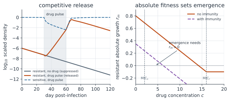
The immune term $aI$ cancels in the selection coefficient $s$, so selection depends only on the drug. But the immune term does not cancel in the absolute growth rate $r_r$, and it is $r_r > 0$, not $s > 0$, that decides whether resistance actually emerges. The two can disagree. At a high concentration the resistant clone can be strongly favored ($s > 0$) yet still shrink ($r_r < 0$) because immunity and the drug together outpace its growth, so there is positive selection but no emergence. The right panel below plots $r_r$ against drug concentration with and without immunity, and the threshold for emergence is where the curve crosses zero, not the MIC.

Competitive release#

The left panel is the mechanism behind the population model’s $\rho\tau$ term. Before treatment the sensitive majority keeps the immune response high, and the resistant clone’s absolute growth rate is negative even though it would be favored under drug. This is competitive suppression, an ecological barrier to resistance rather than a genetic one. A drug pulse removes the sensitive population, the immune pressure relaxes, and the resistant clone’s absolute growth rate turns positive. It then expands, released from the competition that was holding it down. Day, Huijben & Read call this competitive release, and they define it as the change in the resistant clone’s absolute fitness when treatment shifts the within-host environment from its suppressed state $x^\ast$ to its rebounding state $x$,

$$\mathrm{CR} = r_r(c, x) - r_r(c, x^\ast).$$

The lesson runs directly against the naive reading of the mutant selection window (Drlica 2003), which places the lower edge of the dangerous concentration range at the MIC. Competitive release can carry a resistant clone to high density at concentrations below the MIC, because the boundary that matters is set by the host’s ecological state, not by an in-vitro susceptibility number. It also reframes the individual-versus-population tension. The aggressive regimen that most reliably cures the patient is also the one that most completely clears the sensitive competitors, which produces the strongest competitive release for any resistant cell that does exist (Day, Huijben & Read 2015).

In code#

Simulate the within-host model with no drug and with a drug pulse, and confirm the two signatures: selection can be positive while absolute fitness is negative, and the resistant clone is released once the drug removes its competitor.

import numpy as np
from scipy.integrate import solve_ivp

lam_max, lam_r_max, MIC_s, MIC_r = 1.0, 0.9, 2.0, 16.0
a_imm, d_nat, alpha, delta = 0.9, 0.10, 1.0, 1.0

lam_s = lambda c: lam_max * max(0.0, 1 - c / MIC_s)
lam_r = lambda c: lam_r_max * max(0.0, 1 - c / MIC_r)


def within_host(t, y, cfun):
    S, R, I = y
    c = cfun(t)
    dS = (lam_s(c) - a_imm * I - d_nat) * S
    dR = (lam_r(c) - a_imm * I - d_nat) * R
    dI = alpha * (S + R) - delta * I          # immunity tracks total load
    return [dS, dR, dI]


# Selection vs absolute fitness at a high concentration, with immunity I=0.56.
c, I = 8.0, 0.56
s = lam_r(c) - lam_s(c)
r_r = lam_r(c) - a_imm * I - d_nat
print(f"at c={c}: selection s={s:+.3f} (favors resistance), "
      f"absolute r_r={r_r:+.3f}")

# Competitive release: resistant peak with no drug vs a drug pulse.
y0 = [1.0, 1e-6, 1.0]                          # rare resistant clone
no_drug = solve_ivp(within_host, [0, 120], y0, args=(lambda t: 0.0,),
                    dense_output=False, rtol=1e-9, atol=1e-12)
pulse = lambda t: 6.0 if 30.0 <= t <= 60.0 else 0.0
drug = solve_ivp(within_host, [0, 120], y0, args=(pulse,),
                 rtol=1e-9, atol=1e-12)
print(f"resistant peak  no drug: {no_drug.y[1].max():.2e} (suppressed)")
print(f"resistant peak  pulse:   {drug.y[1].max():.2e} (released)")

at c=8.0: selection s=+0.450 (favors resistance), absolute r_r=-0.154
resistant peak  no drug: 1.00e-06 (suppressed)
resistant peak  pulse:   3.60e-01 (released)

library(deSolve)

lam_max <- 1; lam_r_max <- 0.9; MIC_s <- 2; MIC_r <- 16
a_imm <- 0.9; d_nat <- 0.10; alpha <- 1; delta <- 1

lam_s <- function(c) lam_max * max(0, 1 - c / MIC_s)
lam_r <- function(c) lam_r_max * max(0, 1 - c / MIC_r)

within_host <- function(t, y, p) {
  S <- y[1]; R <- y[2]; I <- y[3]
  c  <- if (p$pulse && t >= 30 && t <= 60) 6 else 0
  dS <- (lam_s(c) - a_imm * I - d_nat) * S
  dR <- (lam_r(c) - a_imm * I - d_nat) * R
  dI <- alpha * (S + R) - delta * I          # immunity tracks total load
  list(c(dS, dR, dI))
}

y0 <- c(S = 1, R = 1e-6, I = 1)
t  <- seq(0, 120, by = 0.1)
no_drug <- ode(y0, t, within_host, list(pulse = FALSE))
pulse   <- ode(y0, t, within_host, list(pulse = TRUE))
c(no_drug = max(no_drug[, "R"]), pulse = max(pulse[, "R"]))   # suppressed vs released

using DifferentialEquations

lam_max, lam_r_max, MIC_s, MIC_r = 1.0, 0.9, 2.0, 16.0
a_imm, d_nat, alpha, delta = 0.9, 0.10, 1.0, 1.0

lam_s(c) = lam_max * max(0.0, 1 - c / MIC_s)
lam_r(c) = lam_r_max * max(0.0, 1 - c / MIC_r)

function within_host!(du, u, pulse, t)
    S, R, I = u
    c = (pulse && 30 <= t <= 60) ? 6.0 : 0.0
    du[1] = (lam_s(c) - a_imm * I - d_nat) * S
    du[2] = (lam_r(c) - a_imm * I - d_nat) * R
    du[3] = alpha * (S + R) - delta * I        # immunity tracks total load
end

y0 = [1.0, 1e-6, 1.0]
no_drug = solve(ODEProblem(within_host!, y0, (0.0, 120.0), false), Tsit5())
pulse   = solve(ODEProblem(within_host!, y0, (0.0, 120.0), true),  Tsit5())
(maximum(u[2] for u in no_drug.u), maximum(u[2] for u in pulse.u))  # suppressed vs released

Joining the scales: a nested malaria model#

The two scales meet in the currency the population model took as given. Within-host competition and release decide how many resistant cells a treated host carries; how many transmissible forms those cells produce decides how much resistance that host passes on. Malaria makes this concrete, and it is the system in which competitive release was measured, so it is the natural place to close the loop, following Mideo & Day (2008).

Inside the host, sensitive and resistant asexual parasites, $P_s$ and $P_r$, compete for a shared pool of red blood cells $R$. A fraction of asexual parasites convert to transmissible sexual forms, the gametocytes $G_s$ and $G_r$, at rate $g$. The resistant strain pays a growth cost, so $b_r = b_s(1-c)$, and treatment kills only sensitive asexuals, at rate $k(t)$ during the drug pulse.

$$\begin{aligned} \frac{dR}{dt} &= \Lambda - \mu R - \psi R (P_s + P_r) \\ \frac{dP_s}{dt} &= b_s\, \psi R P_s - dP_s - gP_s - k(t) P_s \\ \frac{dP_r}{dt} &= b_r\, \psi R P_r - dP_r - gP_r \\ \frac{dG_s}{dt} &= g P_s - \mu_g G_s, \qquad \frac{dG_r}{dt} = g P_r - \mu_g G_r \end{aligned}$$

The shared red-cell pool is the competition, and it is exactly what produces competitive release. When the sensitive strain is common it draws $R$ down, and the resistant strain, carrying a cost, cannot grow. A drug pulse crashes $P_s$, red cells rebound, and $P_r$ is released, exactly as in the abstract within-host model but now with an explicit resource.

Gametocytes are the bridge to the next scale. A host with gametocyte density $G$ transmits to a biting mosquito with a probability that saturates as gametocytes become plentiful,

$$\beta(G) = \beta_{\max}\,\frac{G}{G + G_{50}}.$$

Integrating each strain’s gametocyte density over the course of an infection gives a transmissibility weight, and those weights are the between-host transmission rates $\beta_s$ and $\beta_r$ that the two-strain population model needs. The share of a treated host’s gametocyte output that is resistant is the release probability $\rho$ that seeds resistance de novo at the population scale. The between-host layer is the same SIS system as before, now with every rate handed up from the within-host model.

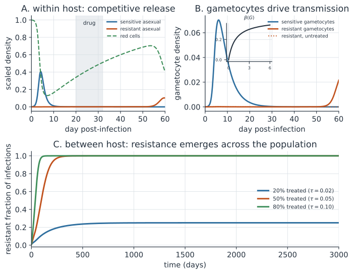
The nested model earns two things the single-scale models could only assume. The de novo rate $\rho\tau$ is no longer a free parameter; it is computed from how much resistant gametocytemia a treated infection produces through competitive release. And the whole individual-versus-population tension becomes a single mechanism seen at two scales. Treating a larger share of infections cures more patients now, and each cure clears sensitive competitors, releases resistant gametocytes, and raises the resistant fraction of transmission, so the population-scale resistant sweep in panel C is the aggregate shadow of the within-host release in panel A.

Reproductive restraint#

The conversion rate $g$ is not a constant the parasite is stuck with. Malaria parasites convert only a small percentage of asexual forms to gametocytes, and they adjust that percentage in response to how their asexual population is faring. Mideo & Day (2008) framed this apparent reproductive restraint as a life-history trade-off between transmitting now and surviving within the host to transmit later, the malaria version of the life-history logic that governs age at maturity in any organism. When a drug knocks down the asexual population, the parasite’s best response can flip from restraint to terminal investment, raising conversion to salvage transmission from a losing infection (Schneider et al. 2018). That plasticity means a treated host can shed more transmissible forms per parasite than an untreated one, which is a within-host behavior that changes the between-host transmission of resistance, and a reason the coupling in the figure is not a one-way street.

In code#

Build the within-host malaria model, derive the transmission rates and the release probability from gametocyte output, and feed them into the between-host SIS layer to recover the resistant sweep.

import numpy as np
from scipy.integrate import solve_ivp

muR, Lam, psi, b_s, cost = 0.025, 0.025, 2.0, 1.5, 0.15
b_r = b_s * (1 - cost)
dp, gconv, mug, kmax = 1.0, 0.10, 0.25, 6.0


def within(t, y, treat):
    R, Ps, Pr, Gs, Gr = y
    k = kmax if (treat and 20.0 <= t <= 32.0) else 0.0
    inf_s, inf_r = psi * R * Ps, psi * R * Pr
    return [Lam - muR * R - inf_s - inf_r,
            b_s * inf_s - dp * Ps - gconv * Ps - k * Ps,
            b_r * inf_r - dp * Pr - gconv * Pr,
            gconv * Ps - mug * Gs,
            gconv * Pr - mug * Gr]


t_eval = np.linspace(0, 60, 1200)
auc = lambda t, g: np.trapezoid(np.clip(g, 0, None), t)
# Strain-dominant untreated infections set each transmission rate.
s_dom = solve_ivp(within, [0, 60], [1, 1e-3, 0, 0, 0], args=(False,),
                  t_eval=t_eval, rtol=1e-9, atol=1e-12)
r_dom = solve_ivp(within, [0, 60], [1, 0, 1e-3, 0, 0], args=(False,),
                  t_eval=t_eval, rtol=1e-9, atol=1e-12)
# A mixed, treated infection sets the release probability.
mix_t = solve_ivp(within, [0, 60], [1, 1e-3, 1e-5, 0, 0], args=(True,),
                  t_eval=t_eval, rtol=1e-9, atol=1e-12)

kappa, gamma_h = 0.31, 0.10
beta_s = kappa * auc(s_dom.t, s_dom.y[3])
beta_r = kappa * auc(r_dom.t, r_dom.y[4])
Gs_m, Gr_m = auc(mix_t.t, mix_t.y[3]), auc(mix_t.t, mix_t.y[4])
rho = Gr_m / (Gs_m + Gr_m)
print(f"beta_s={beta_s:.3f} (R_s={beta_s/gamma_h:.2f})  "
      f"beta_r={beta_r:.3f} (R_r={beta_r/gamma_h:.2f})  release rho={rho:.3f}")


def between(t, y, tau):
    S, Is, Ir = y
    ns, nr = beta_s * S * Is, beta_r * S * Ir
    return [gamma_h * (Is + Ir) + (1 - rho) * tau * Is - ns - nr,
            ns - gamma_h * Is - tau * Is,
            nr - gamma_h * Ir + rho * tau * Is]


for tau, lab in [(0.02, "20% treated"), (0.05, "50%"), (0.10, "80%")]:
    sol = solve_ivp(between, [0, 3000], [0.98, 0.01, 1e-4],
                    args=(tau,), rtol=1e-9, atol=1e-12)
    S, Is, Ir = sol.y[:, -1]
    print(f"{lab:12s} tau={tau:.2f}  resistant fraction={Ir/(Is+Ir):.3f}")

beta_s=0.252 (R_s=2.52)  beta_r=0.199 (R_r=1.99)  release rho=0.086
20% treated  tau=0.02  resistant fraction=0.250
50%          tau=0.05  resistant fraction=1.000
80%          tau=0.10  resistant fraction=1.000

library(deSolve)

muR <- 0.025; Lam <- 0.025; psi <- 2; b_s <- 1.5; cost <- 0.15
b_r <- b_s * (1 - cost)
dp <- 1; gconv <- 0.10; mug <- 0.25; kmax <- 6

within <- function(t, y, p) {
  R <- y[1]; Ps <- y[2]; Pr <- y[3]; Gs <- y[4]; Gr <- y[5]
  k <- if (p$treat && t >= 20 && t <= 32) kmax else 0
  inf_s <- psi * R * Ps; inf_r <- psi * R * Pr
  list(c(Lam - muR * R - inf_s - inf_r,
         b_s * inf_s - dp * Ps - gconv * Ps - k * Ps,
         b_r * inf_r - dp * Pr - gconv * Pr,
         gconv * Ps - mug * Gs,
         gconv * Pr - mug * Gr))
}

t   <- seq(0, 60, by = 0.05)
auc <- function(tt, g) sum(diff(tt) * (head(pmax(g, 0), -1) +
                                       tail(pmax(g, 0), -1)) / 2)
s_dom <- ode(c(1, 1e-3, 0, 0, 0), t, within, list(treat = FALSE))
r_dom <- ode(c(1, 0, 1e-3, 0, 0), t, within, list(treat = FALSE))
mix_t <- ode(c(1, 1e-3, 1e-5, 0, 0), t, within, list(treat = TRUE))

kappa <- 0.31; gamma_h <- 0.10
beta_s <- kappa * auc(s_dom[, 1], s_dom[, 5])   # sensitive gametocytes
beta_r <- kappa * auc(r_dom[, 1], r_dom[, 6])   # resistant gametocytes
rho <- auc(mix_t[, 1], mix_t[, 6]) /
       (auc(mix_t[, 1], mix_t[, 5]) + auc(mix_t[, 1], mix_t[, 6]))

between <- function(t, y, p) {
  S <- y[1]; Is <- y[2]; Ir <- y[3]; tau <- p$tau
  ns <- beta_s * S * Is; nr <- beta_r * S * Ir
  list(c(gamma_h * (Is + Ir) + (1 - rho) * tau * Is - ns - nr,
         ns - gamma_h * Is - tau * Is,
         nr - gamma_h * Ir + rho * tau * Is))
}
frac <- function(tau) {
  out <- ode(c(0.98, 0.01, 1e-4), seq(0, 3000, 5), between, list(tau = tau))
  last <- out[nrow(out), ]
  last[4] / (last[3] + last[4])
}
sapply(c(0.02, 0.05, 0.10), frac)

using DifferentialEquations

muR, Lam, psi, b_s, cost = 0.025, 0.025, 2.0, 1.5, 0.15
b_r = b_s * (1 - cost)
dp, gconv, mug, kmax = 1.0, 0.10, 0.25, 6.0

function within!(du, u, treat, t)
    R, Ps, Pr, Gs, Gr = u
    k = (treat && 20 <= t <= 32) ? kmax : 0.0
    inf_s, inf_r = psi * R * Ps, psi * R * Pr
    du[1] = Lam - muR*R - inf_s - inf_r
    du[2] = b_s*inf_s - dp*Ps - gconv*Ps - k*Ps
    du[3] = b_r*inf_r - dp*Pr - gconv*Pr
    du[4] = gconv*Ps - mug*Gs
    du[5] = gconv*Pr - mug*Gr
end

auc(sol, idx) = sum((sol.t[i+1]-sol.t[i]) *
    (max(sol.u[i][idx],0)+max(sol.u[i+1][idx],0))/2 for i in 1:length(sol.t)-1)
grid = 0:0.05:60
s_dom = solve(ODEProblem(within!, [1,1e-3,0,0,0], (0.0,60.0), false), Tsit5(); saveat=grid)
r_dom = solve(ODEProblem(within!, [1,0,1e-3,0,0], (0.0,60.0), false), Tsit5(); saveat=grid)
mix_t = solve(ODEProblem(within!, [1,1e-3,1e-5,0,0], (0.0,60.0), true), Tsit5(); saveat=grid)

kappa, gamma_h = 0.31, 0.10
beta_s = kappa * auc(s_dom, 4)
beta_r = kappa * auc(r_dom, 5)
rho = auc(mix_t, 5) / (auc(mix_t, 4) + auc(mix_t, 5))

function between!(du, u, tau, t)
    S, Is, Ir = u
    ns, nr = beta_s*S*Is, beta_r*S*Ir
    du[1] = gamma_h*(Is+Ir) + (1-rho)*tau*Is - ns - nr
    du[2] = ns - gamma_h*Is - tau*Is
    du[3] = nr - gamma_h*Ir + rho*tau*Is
end
frac(tau) = (u = solve(ODEProblem(between!, [0.98,0.01,1e-4], (0.0,3000.0), tau),
                       Tsit5(); reltol=1e-9).u[end]; u[3]/(u[2]+u[3]))
frac.((0.02, 0.05, 0.10))

Why it matters#

Resistance looks like two contradictory problems only until the scales are joined. The clinician who treats hard is right that it cures the patient, and the steward who worries about aggregate use is right that it drives resistance, and the nested model shows these are the same act seen from two distances. Aggressive treatment clears sensitive competitors, which releases resistant cells inside the host, which shed more resistant transmissible forms, which raise the resistant fraction circulating in the population. Naming the mechanism at each scale is what turns “use antibiotics wisely” into specific, testable levers. Keep the resistant clone’s absolute fitness negative rather than merely disfavored (Day, Huijben & Read 2015); preserve enough competitive suppression that release never fires; and remember that the community treatment rate, not any single prescription, sits on the population-scale threshold $\tau^\ast$. The same cross-scale reasoning underlies resistance management in cancer chemotherapy and herbicide use, wherever a treatment that helps the individual target erodes a resource shared by many.

Related#

• Population Dynamics of Resistance — the two-strain competition and treatment threshold in isolation
• The Evolution of Resistance — within-host selection and the cost of resistance
• Nested Within- and Between-Host Models — the cross-scale nesting for virulence, the same machinery applied here
• Within-Host Dynamics and the Immune Response — the target-cell model behind the individual scale
• Antimicrobial PK/PD — the MIC, the mutant selection window, and dosing in one patient
• Adaptive Dynamics and the Evolution of Virulence — trade-offs and singular strategies across scales
• The Price Equation and Evolutionary Epidemiology — partitioning selection into within- and between-host components
• Life-History Theory — the trade-off behind reproductive restraint
• Cost-Effectiveness Analysis — valuing the shared drug resource across a population
• Quantitative Methods