Approximate Bayesian Computation

Some models are easy to simulate but impossible to write a likelihood for. A stochastic transmission model, a phylodynamic process, an agent-based simulation — you can run them forward and generate data, but the probability of any particular dataset has no closed form. Approximate Bayesian Computation (ABC) fits exactly these models, replacing the intractable likelihood with simulation: propose parameters, simulate data, and keep the parameters whose simulations look like what you observed.

The likelihood-free idea#

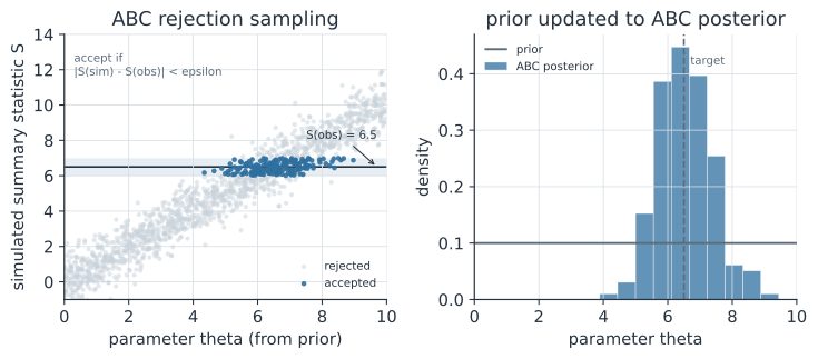
Bayesian inference wants the posterior $p(\theta \mid y) \propto p(y \mid \theta)\, p(\theta)$, but here the likelihood $p(y \mid \theta)$ cannot be evaluated. ABC’s insight is that you do not need to evaluate the likelihood if you can sample from it, because running the simulator with parameter $\theta$ is drawing from $p(y \mid \theta)$. The basic rejection ABC algorithm is three steps repeated many times:

1. Propose $\theta^\* \sim p(\theta)$ from the prior.
2. Simulate a dataset $y^\* \sim p(y \mid \theta^\*)$ by running the model.
3. Accept $\theta^\*$ if the simulated data are close enough to the observed, $\rho\big(S(y^\*), S(y)\big) < \varepsilon$.

The accepted parameters are a sample from an approximation to the posterior, and the approximation becomes exact as the tolerance $\varepsilon \to 0$ and the summary is sufficient.

Summary statistics and the tolerance#

Two choices control everything. Comparing whole datasets directly is hopeless, so ABC compares low-dimensional summary statistics $S(y)$ — an epidemic’s growth rate, peak time, and final size, say, rather than the full case time series. If the summaries are sufficient they lose no information and ABC targets the true posterior; in practice they are chosen to be informative but not sufficient, which is the main source of ABC’s approximation error. The tolerance $\varepsilon$ sets a bias-variance trade-off: a tight tolerance gives a more accurate posterior but accepts almost nothing, wasting simulations, while a loose tolerance accepts many but smears the posterior toward the prior.

The curse of dimensionality#

The reason ABC leans so hard on summaries is that acceptance collapses as the dimension of the comparison grows. Requiring a high-dimensional simulated dataset to fall within $\varepsilon$ of the observed in every coordinate becomes astronomically unlikely, so the acceptance rate crashes and the method becomes unusable. Reducing the data to a handful of summaries keeps the comparison in a low enough dimension that a workable fraction of simulations are accepted — the whole reason summaries are not optional.

Beyond rejection#

Rejection ABC wastes most of its simulations on parameters the prior likes but the data do not. ABC-MCMC and sequential Monte Carlo ABC (ABC-SMC) concentrate effort where it matters: ABC-SMC evolves a population of parameter particles through a decreasing sequence of tolerances, each round resampling and perturbing the survivors so proposals home in on the high-posterior region (Toni et al. 2009). Related refinements weight accepted parameters by how close their simulations landed and regression-adjust them toward the observed summary (Beaumont et al. 2002). These make ABC practical for the stochastic dynamical models — including epidemic and phylodynamic models — where it is often the only feasible route to a posterior, a likelihood-free counterpart to the particle filter.

A worked example#

We infer one parameter of a model whose summary statistic is the parameter plus noise. Rejection ABC draws from a uniform prior, simulates the summary, and keeps draws within a tolerance of the observed value.

In code#

R#

set.seed(1834)
s_obs <- 6.5; eps <- 0.5; n <- 200000

theta <- runif(n, 0, 10)                 # prior draws
s_sim <- theta + rnorm(n, 0, 0.8)        # simulate the summary statistic
accepted <- theta[abs(s_sim - s_obs) < eps]

c(n_accepted = length(accepted),
  post_mean = mean(accepted), post_sd = sd(accepted))

Python#

import numpy as np

rng = np.random.default_rng(1834)
s_obs, eps, n = 6.5, 0.5, 200_000

theta = rng.uniform(0, 10, n)            # prior draws
s_sim = theta + rng.normal(0, 0.8, n)    # simulate the summary statistic
accepted = theta[np.abs(s_sim - s_obs) < eps]

print(f"accepted        = {accepted.size} of {n}")
print(f"posterior mean  = {accepted.mean():.3f}")
print(f"posterior sd    = {accepted.std():.3f}")

accepted        = 19894 of 200000
posterior mean  = 6.487
posterior sd    = 0.852

Julia#

using Random, Statistics

Random.seed!(1834)
s_obs, eps, n = 6.5, 0.5, 200_000

theta = rand(n) .* 10                    # prior draws on (0, 10)
s_sim = theta .+ randn(n) .* 0.8         # simulate the summary statistic
accepted = theta[abs.(s_sim .- s_obs) .< eps]

(n_accepted = length(accepted), post_mean = mean(accepted),
 post_sd = std(accepted))

The accepted parameters concentrate near the value of $\theta$ consistent with the observed summary, turning a flat prior into a peaked posterior using only forward simulation.

Fitting an SIR with ABC-SMC#

The toy model above has a one-line simulator; the point of ABC is fitting models that do not. Here we infer the basic reproduction number $R_0$ of a stochastic SIR epidemic from a single observed outbreak, using sequential Monte Carlo ABC. There is no likelihood — the simulator is a chain-binomial SIR — so every step is driven by forward simulation. We compare epidemics through three summary statistics (the peak size, the day of the peak, and the final attack rate), and let the tolerance tighten to the running median each round while a Gaussian kernel perturbs the surviving particles.

import numpy as np

rng = np.random.default_rng(1834)
N, GAMMA, I0, DAYS = 600, 0.2, 5, 60

def simulate(R0):
    """One stochastic chain-binomial SIR run; return daily incidence."""
    beta = R0 * GAMMA
    S, I = N - I0, I0
    inc = np.empty(DAYS)
    for t in range(DAYS):
        new_inf = rng.binomial(S, 1 - np.exp(-beta * I / N))
        new_rec = rng.binomial(I, GAMMA)
        S -= new_inf
        I += new_inf - new_rec
        inc[t] = new_inf
    return inc

def summary(inc):
    """Peak size, day of the peak, and final attack rate."""
    return np.array([inc.max(), inc.argmax(), inc.sum()])

scale = np.array([40.0, 8.0, 150.0])          # standardize the summaries
y_obs = summary(simulate(2.5))                # observed epidemic, true R0 = 2.5

def distance(R0):
    return np.sqrt(np.sum(((summary(simulate(R0)) - y_obs) / scale) ** 2))

# --- ABC-SMC over a decreasing tolerance schedule ---
n_part, n_rounds, lo, hi = 120, 5, 1.0, 5.0

# Round 0: rejection from the prior, keep the closest n_part draws.
pool = rng.uniform(lo, hi, n_part * 8)
pool_d = np.array([distance(t) for t in pool])
keep = np.argsort(pool_d)[:n_part]
theta, theta_d = pool[keep], pool_d[keep]
w = np.ones(n_part) / n_part

for r in range(1, n_rounds):
    eps = np.median(theta_d)                  # tighten to the current median
    ksd = np.std(theta) + 1e-9                # Gaussian perturbation scale
    new_theta, new_d = np.empty(n_part), np.empty(n_part)
    for i in range(n_part):
        for _ in range(3000):                 # safety cap on proposals
            cand = theta[rng.choice(n_part, p=w)] + rng.normal(0, ksd)
            if lo <= cand <= hi and distance(cand) < eps:
                new_theta[i] = cand
                new_d[i] = distance(cand)
                break
        else:
            new_theta[i], new_d[i] = theta[i], theta_d[i]   # fallback
    # Importance weights (uniform prior, so the numerator is constant).
    kern = np.exp(-0.5 * ((new_theta[:, None] - theta[None, :]) / ksd) ** 2)
    w = 1.0 / (kern @ w)
    w /= w.sum()
    theta, theta_d = new_theta, new_d

resample = rng.choice(theta, size=5000, p=w)  # weighted posterior sample
lo95, hi95 = np.quantile(resample, [0.025, 0.975])
print(f"observed summaries (peak, day, size) = {y_obs.astype(int)}")
print(f"ABC-SMC posterior mean R0 = {np.sum(w * theta):.2f}")
print(f"95% credible interval     = ({lo95:.2f}, {hi95:.2f})")

observed summaries (peak, day, size) = [ 40  17 539]
ABC-SMC posterior mean R0 = 2.30
95% credible interval     = (1.72, 3.00)

Starting from a flat prior on $[1, 5]$ and nothing but the ability to simulate epidemics, ABC-SMC recovers a posterior for $R_0$ centered near the value that generated the data, and the shrinking tolerance across rounds is what sharpens it. Swap in a more elaborate simulator — age structure, spatial spread, under-reporting — and the algorithm is unchanged: only simulate and the summaries need to grow.

Why it matters#

ABC extends Bayesian inference to the large class of models that can be simulated but not written down as a likelihood, which includes many of the mechanistic stochastic models epidemiology cares about most. Its accuracy is bought with two approximations that must be watched: the choice of summary statistics, which fixes what information the data can contribute, and the tolerance, which trades bias against how many simulations you can afford. Where a likelihood is available, methods like particle filtering and MCMC are more efficient; ABC is what you reach for when it is not.

Related#

• Bayesian Inference — the posterior ABC approximates
• Markov Chain Monte Carlo — the sampler when a likelihood is available
• State-Space Models and Particle Filtering — the other main route to likelihood-free inference
• Prior Predictive Checks — simulating from the prior, the same forward step ABC uses
• Fitting Dynamic Models to Data — calibration when the likelihood is tractable