State-Space Models and Particle Filtering

Surveillance data are a noisy, partial shadow of the process we actually care about. We see reported cases; we want the underlying transmission dynamics that generated them, through a haze of reporting error, under-ascertainment, and stochastic chance. State-space models formalize this split into a hidden dynamical process and a noisy observation of it, and particle filters are the simulation-based engine that recovers the hidden state and the likelihood — the key that unlocks fitting mechanistic epidemic models to real data.

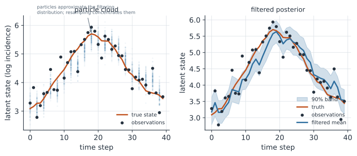
Partially observed Markov processes#

A state-space model, also called a partially observed Markov process (POMP), has two layers. The process model is a Markov transition for the hidden state $x_t$ — an SIR simulation, a stochastic renewal process, a random walk in log-incidence — often without a tractable likelihood because it is defined by a simulator rather than a formula. The observation model links the hidden state to the data, $y_t \sim g(y_t \mid x_t)$, encoding reporting probability, overdispersion, and delay. The inferential problem is that we only see $y_{1:T}$ and must reason about the unobserved $x_{1:T}$ and the parameters governing both layers.

The central quantity is the filtering distribution $p(x_t \mid y_{1:t})$: our belief about the current hidden state given all data so far. For linear-Gaussian models the Kalman filter computes it exactly, and the ensemble Kalman filter extends it approximately to nonlinear models, but epidemic models are nonlinear and non-Gaussian, which is where particle filters come in.

The bootstrap particle filter#

A particle filter represents the filtering distribution by a swarm of particles — sampled state values — that are propagated, weighted, and resampled as each observation arrives. The bootstrap version is three steps per time point:

1. Propagate. Push each particle forward through the process simulator, $x_t^{(i)} \sim f(x_t \mid x_{t-1}^{(i)})$.
2. Weight. Weight each by how well it explains the new observation, $w^{(i)} \propto g(y_t \mid x_t^{(i)})$.
3. Resample. Draw a new set of particles in proportion to the weights, concentrating them where the data say the state is.

The particles approximate the filtering distribution at every step, and the average unnormalized weight at each time gives an unbiased estimate of the likelihood $p(y_{1:T})$ — the piece needed to fit parameters. Only the ability to simulate the process and evaluate the observation density is required; the process likelihood never has to be written down, which is what makes the method work for mechanistic models.

Fitting mechanistic models#

A particle filter estimates the hidden state for fixed parameters; fitting the parameters wraps an optimizer or sampler around it. Iterated filtering perturbs the parameters, runs the filter, and lets the filtering update itself drive the parameters toward the maximum likelihood, repeating with shrinking perturbations until they converge (Ionides et al. 2006). This is the machinery behind the pomp framework, which has become a standard tool for confronting stochastic transmission models with time-series data (King et al. 2016). Alternatively, plugging the particle filter’s unbiased likelihood into an MCMC sampler gives particle MCMC, a fully Bayesian route to the same goal, complementing the calibration methods used when a likelihood is available directly.

A worked example#

We simulate a simple state-space model — a random walk in log-incidence observed with Gaussian noise — and run a bootstrap particle filter to recover the hidden final state and the marginal log-likelihood.

In code#

R#

set.seed(1834)
Tn <- 30; sig_p <- 0.15; sig_o <- 0.25

x <- numeric(Tn)
for (t in 2:Tn) x[t] <- x[t - 1] + rnorm(1, 0, sig_p)
y <- x + rnorm(Tn, 0, sig_o)

N <- 2000
particles <- rnorm(N, 0, 1)
filt <- numeric(Tn); loglik <- 0
for (t in 1:Tn) {
  if (t > 1) particles <- particles + rnorm(N, 0, sig_p)   # propagate
  w <- dnorm(y[t], particles, sig_o)                       # weight
  loglik <- loglik + log(mean(w))
  w <- w / sum(w)
  filt[t] <- sum(w * particles)
  particles <- sample(particles, N, replace = TRUE, prob = w)  # resample
}

round(c(true_final = x[Tn], filtered_final = filt[Tn], loglik = loglik), 3)

Python#

import numpy as np
from scipy.stats import norm

rng = np.random.default_rng(1834)
Tn, sig_p, sig_o = 30, 0.15, 0.25

x = np.zeros(Tn)
for t in range(1, Tn):
    x[t] = x[t - 1] + rng.normal(0, sig_p)
y = x + rng.normal(0, sig_o, Tn)

N = 2000
particles = rng.normal(0, 1, N)
filt = np.zeros(Tn)
loglik = 0.0
for t in range(Tn):
    if t > 0:
        particles = particles + rng.normal(0, sig_p, N)      # propagate
    w = norm.pdf(y[t], particles, sig_o)                     # weight
    loglik += np.log(w.mean())
    w /= w.sum()
    filt[t] = np.sum(w * particles)
    particles = rng.choice(particles, N, replace=True, p=w)  # resample

print(f"true final state     = {x[-1]:.3f}")
print(f"filtered final state = {filt[-1]:.3f}")
print(f"marginal log-likelihood = {loglik:.3f}")

true final state     = 1.147
filtered final state = 1.279
marginal log-likelihood = -11.410

Julia#

using Distributions, Random, StatsBase, Statistics

Random.seed!(1834)
Tn, sig_p, sig_o = 30, 0.15, 0.25

x = zeros(Tn)
for t in 2:Tn
    x[t] = x[t - 1] + rand(Normal(0, sig_p))
end
y = x .+ rand(Normal(0, sig_o), Tn)

N = 2000
particles = rand(Normal(0, 1), N)
filt = zeros(Tn); loglik = 0.0
for t in 1:Tn
    t > 1 && (particles .+= rand(Normal(0, sig_p), N))          # propagate
    w = pdf.(Normal.(particles, sig_o), y[t])                  # weight
    loglik += log(mean(w))
    w ./= sum(w)
    filt[t] = sum(w .* particles)
    particles = sample(particles, Weights(w), N)               # resample
end

(true_final = x[Tn], filtered_final = filt[Tn], loglik = loglik)

Why it matters#

State-space models are the honest way to fit epidemic dynamics, because they keep the mechanism and the messy observation process as separate, explicit layers instead of pretending the data are the truth. The particle filter makes them tractable: as long as you can simulate forward and score an observation, it recovers the hidden states and an unbiased likelihood, even when the process has no closed-form likelihood at all. That combination — mechanistic simulator plus a filter that yields a likelihood — is what lets iterated filtering and particle MCMC fit stochastic transmission models to the surveillance data we actually collect.

Related#

• Fitting Dynamic Models to Data — calibration when a likelihood is available
• Markov Chains — the process layer of a state-space model
• Markov Chain Monte Carlo — the sampler behind particle MCMC
• Stochastic Epidemics and the Gillespie Algorithm — simulating the hidden process
• The Effective Reproduction Number and Forecasting — a common target of state-space inference