Bland–Altman Agreement

Two methods claim to measure the same thing — a new point-of-care assay against a laboratory reference, two devices, two readers. How do you tell whether they agree well enough to be used interchangeably? The instinct is to correlate them, or regress one on the other, and report a high $r$. That instinct is wrong: correlation measures whether two quantities move together, not whether they agree, and a badly biased method can still correlate almost perfectly with the truth. The Bland–Altman method (Bland & Altman, 1986) answers the real question directly.

Why not correlation (or regression)?#

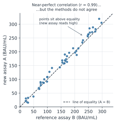
Correlation is the wrong tool for three reasons (Figure 1):

• It rewards range, not agreement. Spread your samples over a wide range of true values and $r \to 1$ almost regardless of how the methods differ.
• It is blind to bias. Add a constant to every reading of one method and the correlation is unchanged, even though the methods now disagree by that amount everywhere.
• A significance test of $r$ answers a pointless question — that the two methods are related, which we already knew because they measure the same thing.

Regressing one method on the other is only a little better and invites the same misreading. The question is not “are they associated?” but “how far apart are a method’s readings from the other’s, and is that gap small enough to ignore?”

Differences versus means#

Bland–Altman reframes the comparison around the two quantities that matter. For each subject $i$ with paired measurements $A_i$ and $B_i$, form the difference and the mean:

$$d_i = A_i - B_i, \qquad m_i = \frac{A_i + B_i}{2}.$$

Plotting $d_i$ against $m_i$ — not $A$ against $B$ — puts disagreement on the vertical axis and magnitude on the horizontal, so both the size of the discrepancies and any dependence on the measurement level become visible. The bias is the mean difference $\bar d$, and its scatter is the standard deviation $s_d$ of the differences.

Limits of agreement#

If the differences are roughly Normal, then 95% of them fall within $\bar d \pm 1.96\, s_d$. These two values are the 95% limits of agreement:

$$\text{LoA} = \bar d \pm 1.96\, s_d. \tag{1}$$

They are a statement about individuals: for a new subject, the two methods will differ by something inside this interval 95% of the time. Whether that width is acceptable is a clinical or scientific judgement, not a statistical one — a ±20 BAU/mL disagreement might be fine for screening and useless for titre monitoring. Because $\bar d$ and $s_d$ are themselves estimated, each limit carries a confidence interval of roughly $\pm t_{n-1}\sqrt{3 s_d^2 / n}$; report it when $n$ is small.

A worked example#

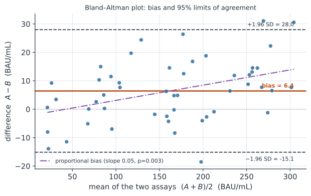
Fifty samples are measured by a new antibody assay ($A$) and a reference assay ($B$). The differences reveal a small positive bias with wide limits of agreement — and, on inspection, a proportional bias: the gap grows with concentration, so the disagreement is worse exactly where the values are largest (Figure 2).

import numpy as np
from scipy import stats

rng = np.random.default_rng(7)
n = 50
true = rng.uniform(20, 300, n)                       # unobserved true value
B = true + rng.normal(0, 6, n)                        # reference assay
A = true + 8 + 0.05 * (true - 160) + rng.normal(0, 8, n)   # new assay (biased)

diff = A - B
avg = (A + B) / 2
bias = diff.mean()
sd = diff.std(ddof=1)
loa_lo, loa_hi = bias - 1.96 * sd, bias + 1.96 * sd

# proportional bias: regress the difference on the mean
slope, intercept, r, p, se = stats.linregress(avg, diff)
r_ab = np.corrcoef(A, B)[0, 1]                        # the misleading number

print(f"bias {bias:.1f}  95% limits of agreement [{loa_lo:.1f}, {loa_hi:.1f}]")
print(f"proportional-bias slope {slope:.3f} (p={p:.3f})")
print(f"correlation r(A,B) = {r_ab:.3f}  <- high, yet the methods disagree")

bias 6.4  95% limits of agreement [-15.1, 28.0]
proportional-bias slope 0.054 (p=0.003)
correlation r(A,B) = 0.993  <- high, yet the methods disagree

The correlation is $0.99$ — the number you would proudly report if you stopped there — while the limits of agreement say two readings of the same sample can differ by more than $40$ BAU/mL across the range. The significant slope confirms the bias is not constant, a signal to model the difference or to analyse on the log scale.

Patterns to look for#

The plot is diagnostic; the shape of the cloud tells you what to do next:

• Constant bias — the cloud is centred away from zero: the methods differ by a fixed offset (recalibrate).
• Proportional bias — the cloud tilts (significant slope of $d$ on $m$): the offset scales with magnitude; model it, or transform.
• Funnelling (heteroscedasticity) — the spread widens with the mean: the differences are not constant-variance, so plain limits of agreement mislead. A log transformation of both methods often fixes this, turning the limits into ratios.
• Repeated measures — several pairs per subject inflate precision if treated as independent; use the version of the method that accounts for within-subject replication.

In code#

R#

d <- A - B
m <- (A + B) / 2
bias <- mean(d); s <- sd(d)
loa <- bias + c(-1, 1) * 1.96 * s
# base-R plot; the blandr / BlandAltmanLeh packages add CIs and proportional-bias tests
plot(m, d, xlab = "mean of methods", ylab = "difference")
abline(h = c(bias, loa), lty = c(1, 2, 2))

Python#

# reuses the arrays above; a compact reusable helper
def bland_altman(a, b):
    d, m = a - b, (a + b) / 2
    bias, s = d.mean(), d.std(ddof=1)
    return bias, (bias - 1.96 * s, bias + 1.96 * s)

Julia#

d = A .- B
m = (A .+ B) ./ 2
bias = mean(d); s = std(d)
loa = (bias - 1.96s, bias + 1.96s)

Why it matters#

Method-comparison studies are everywhere in infectious-disease work: a rapid point-of-care test against a laboratory gold standard, a new PCR platform against an established one, a wearable against a clinical thermometer, two serological assays reporting “the same” antibody titre. Reporting a correlation in these settings is a classic and consequential mistake — it can wave through a device that is biased or wildly variable at the values that matter. Bland–Altman keeps the analysis honest by asking the operational question directly: how far apart are the two methods for an individual, and is that gap tolerable? It is the agreement analogue of the distinction, elsewhere on this site, between a good diagnostic test and a merely correlated one.

Related#

• Diagnostic Testing
• Measures of Variability
• Linear Regression
• Confidence Intervals
• Meta-Analysis
• Quantitative Methods