Capture-Recapture and Multiplier Methods
Surveillance never sees everyone. Cases go undiagnosed, hidden populations avoid contact with services, and no single list is complete. Capture-recapture turns this into a solvable problem: if you have two or more incomplete lists of the same population, the overlap between them tells you how much you are missing, and lets you estimate the true total — including the people on no list at all. Borrowed from ecology, where it estimates animal abundance from tag-and-recapture, it is now a standard tool for correcting undercounts in epidemiology.
The two-source estimator#
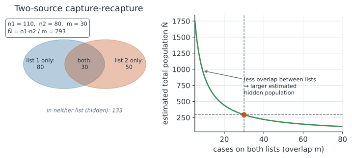
Suppose two independent sources ascertain cases of the same condition: on the first list, on the second, and appearing on both. If the second list samples the population at random, the fraction of the first list that it recaptures, , should equal the fraction of the whole population it captured, . Setting these equal and solving gives the Lincoln-Petersen estimator
The intuition is that small overlap means each list caught a different slice of a large population, so the total is large; heavy overlap means the lists keep finding the same people, so the population is nearly exhausted. Because is unstable and biased upward when is small, the bias-corrected Chapman estimator is preferred in practice,
and it comes with a variance formula for a confidence interval.
The assumptions#
The estimate is only as good as four assumptions, and each maps to a real threat. The population must be closed (no births, deaths, or migration during ascertainment). The lists must be independent — being on one list should not change the chance of being on another, which fails badly when, say, a positive test triggers entry on multiple registries. Individuals must have equal catchability, or at least heterogeneity that the model accounts for, since if some people are systematically hard to capture on every list the method underestimates the hidden group. And records must be matched correctly, because both missed matches and false matches bias the overlap that the whole estimate pivots on. Dependence between sources is usually the most damaging violation, and it is the reason two lists are rarely enough.
More than two sources#
With three or more sources the counts form a contingency table with one missing cell — the people on no list — and the tool becomes a log-linear model fit to the observed cells and extrapolated to the missing one (Hook and Regal 1995). The great advantage is that log-linear models can include interaction terms for dependence between sources, relaxing the independence assumption that cripples the two-source case, and model selection chooses which dependencies the data support. This three-source, log-linear form is the workhorse for estimating hidden and hard-to-reach populations — people who inject drugs, undiagnosed infections, undocumented deaths.
Multiplier methods#
A lighter-weight cousin is the multiplier method: if a benchmark count (say, hospitalizations) is known and an independent survey estimates the fraction of the target population captured by that benchmark, dividing the benchmark by the fraction scales it up to the total. It is the same borrowing-of-strength between two data sources, and it is widely used to size key populations for HIV programs when a full capture-recapture is not feasible.
A worked example#
From two case lists with a known overlap, we compute the Lincoln-Petersen and bias-corrected Chapman estimates and a confidence interval for the total.
In code#
R#
n1 <- 110; n2 <- 80; m <- 30      # list 1, list 2, and both

petersen <- n1 * n2 / m
chapman  <- (n1 + 1) * (n2 + 1) / (m + 1) - 1
var_c <- (n1 + 1) * (n2 + 1) * (n1 - m) * (n2 - m) / ((m + 1)^2 * (m + 2))
ci <- chapman + c(-1.96, 1.96) * sqrt(var_c)

round(c(petersen = petersen, chapman = chapman,
        lower = ci[1], upper = ci[2]))
Python#
import numpy as np

n1, n2, m = 110, 80, 30           # list 1, list 2, and both

petersen = n1 * n2 / m
chapman = (n1 + 1) * (n2 + 1) / (m + 1) - 1
var_c = (n1 + 1) * (n2 + 1) * (n1 - m) * (n2 - m) / ((m + 1) ** 2 * (m + 2))
lo, hi = chapman - 1.96 * np.sqrt(var_c), chapman + 1.96 * np.sqrt(var_c)

print(f"Lincoln-Petersen = {petersen:.0f}")
print(f"Chapman estimate = {chapman:.0f}")
print(f"95% CI           = ({lo:.0f}, {hi:.0f})")
Lincoln-Petersen = 293
Chapman estimate = 289
95% CI           = (222, 356)
Julia#
n1, n2, m = 110, 80, 30           # list 1, list 2, and both

petersen = n1 * n2 / m
chapman  = (n1 + 1) * (n2 + 1) / (m + 1) - 1
var_c = (n1 + 1) * (n2 + 1) * (n1 - m) * (n2 - m) / ((m + 1)^2 * (m + 2))
lo, hi = chapman - 1.96 * sqrt(var_c), chapman + 1.96 * sqrt(var_c)

(petersen = petersen, chapman = chapman, lower = lo, upper = hi)
The two lists together name 160 distinct people, but the overlap implies a total near 290, so roughly 130 cases appear on neither list.
Why it matters#
Capture-recapture is how epidemiology puts a number on what it cannot see, turning the overlap between imperfect data sources into an estimate of the whole, including the part no source touched. Its power is entirely contingent on its assumptions, and the most dangerous — source dependence — is precisely why serious applications use three or more lists and log-linear models rather than a single ratio. Alongside excess mortality, it is one of the two main ways to recover the counts that routine surveillance systematically misses.
Related#
- Survey Sampling — the design-based view of estimating population quantities
- Generalized Linear Models — the log-linear models used for three or more sources
- Maximum Likelihood Estimation — how the estimators are derived
- Severity: Estimating the CFR and IFR — where undercount correction feeds severity
- Excess Mortality — another correction for what surveillance misses