Modern Coexistence Theory and the Storage Effect

Why do competing species so often persist together when simple theory says the better competitor should win? Modern coexistence theory answers by decomposing each species’ growth rate when rare into two parts: stabilizing niche differences that pull rare species back up, and equalizing fitness differences that decide who wins if stabilization is weak. Its most striking result is that a fluctuating environment is not just noise to be averaged away — through the storage effect, variation itself can generate the negative frequency dependence that holds a community together.

Modern coexistence theory: the stabilizing-equalizing plane showing the coexistence region as a function of niche overlap and fitness ratio, and a storage-effect simulation where buffered species have positive low-density growth but unbuffered ones do not.

The invasion criterion

The organizing principle is mutual invasibility: a set of species coexists if each one can increase from low density when the others are at their long-run abundances. Formally, hold species $i$ rare and let the residents settle to their stationary dynamics, then ask whether the invader’s long-run average per-capita growth rate is positive,

$\bar{r}_i \;=\; \big\langle\, \tfrac{1}{N_i}\tfrac{\mathrm{d}N_i}{\mathrm{d}t} \,\big\rangle \;>\; 0 \quad\text{for every } i .$

This is the same mutual-invasibility idea developed for deterministic Lotka–Volterra competition, where two species coexist when each invades the other’s monoculture. Modern coexistence theory keeps the criterion but sharpens the question: it asks what makes $\bar{r}_i$ positive, and it works when the environment varies so that averaging over time cannot be skipped.

Stabilizing versus equalizing

Chesson’s central move (Chesson 2000 doi:10.1086/286080) is to split the invasion growth rate into two additive contributions,

$\bar{r}_i \;\approx\; \underbrace{(\kappa_i-\bar{\kappa})}_{\text{fitness difference}} \;+\; \underbrace{A_i}_{\text{stabilizing term}} .$

The first term is the species’ fitness difference from the community average: on its own it favors whichever competitor has the higher intrinsic fitness and drives the others out. The second is the stabilizing term, the part of low-density growth that comes from negative frequency dependence — a species does better when rare than when common because it limits itself more than it limits others.

Equalizing mechanisms shrink the fitness differences $(\kappa_i-\bar{\kappa})$ , making species more alike in competitive ability. Stabilizing mechanisms raise $A_i$ by strengthening self-limitation relative to cross-limitation, which is what makes rare species recover. The two are not interchangeable: equalizing alone only delays exclusion, because whoever is even slightly fitter still wins eventually, whereas stabilization creates a genuine restoring force. The practical statement is that stronger stabilization lets a community tolerate larger fitness differences — coexistence needs the niche difference to outweigh the fitness gap.

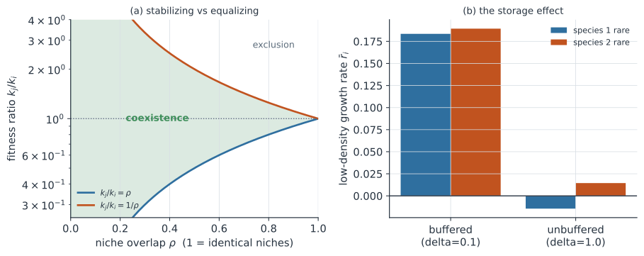
The niche-overlap picture makes this visible. Write the fitness ratio between two species as $k_j/k_i$ and their niche overlap as $\rho\in[0,1]$ , where $\rho=1$ means identical resource use and $\rho=0$ means fully separate niches. Coexistence holds when $\rho < k_j/k_i < 1/\rho$ : less overlap widens the window of fitness ratios that still coexist, so the coexistence region in the plane fans out as niches diverge.

The storage effect

The storage effect is a stabilizing mechanism that exists only because the environment fluctuates, and it needs three ingredients together (Chesson 2000).

Species-specific responses to the environment. Good years for one species are not identical to good years for another, so their environmental responses differ.
Covariance between environment and competition. When a species is common it experiences its own good years crowded with conspecifics, so favorable environment and strong competition coincide; when rare, its good years are relatively uncrowded.
Buffered population growth. A dormant or long-lived stage — a seed bank, a resting egg, a perennial adult — carries the population through bad years so that losses in poor conditions are capped.

Put these together and a rare species reaps its good years with little competition while a common species has its good years eroded by self-competition, which is exactly the negative frequency dependence coexistence needs. The mechanism lives in the covariance term $\operatorname{Cov}(E,C)$ between the environmental response $E$ and the competition it induces $C$ : buffering keeps the invader from paying the full cost of bad years, so its lower environment-competition covariance turns into a positive contribution to $\bar{r}_i$ . Without the buffer — if the whole population turns over every step — the good and bad years cancel in the long-run growth rate and the storage effect vanishes. This is why the buffer is load-bearing, and it ties the mechanism to long-lived stages and their reproductive value: the storage effect is stored in the individuals that persist across the variation.

Relative nonlinearity

The storage effect is not the only fluctuation-dependent mechanism. Relative nonlinearity arises when species differ in the curvature of their growth response to a fluctuating resource or competition variable: a species with a more strongly concave response is penalized by variance in that variable, while a species with a less concave response can exploit it. If one species tends to generate fluctuations and another is better able to tolerate them, the two can coexist on the pattern of variation itself. It is usually weaker than the storage effect in practice, but it completes the point that environmental variation supplies mechanisms of coexistence, not merely obstacles to it.

A worked example

A two-species lottery model makes the storage effect concrete. Each year an environmental draw sets each species’ per-capita reproduction $B_i$ , the two responses are negatively correlated (correlation $-0.8$ , so their good years differ), and a fraction $1-\delta$ of adults survives to buffer growth. The invader’s long-run growth rate is $\bar{r}_i=\big\langle\log\!\big[(1-\delta)+\delta\,B_i/B_{\text{res}}\big]\big\rangle$ , evaluated with species $i$ rare against an established resident. With strong buffering ( $\delta=0.1$ , so $90\%$ of adults survive each year) both species have clearly positive low-density growth, $\bar{r}_1\approx+0.18$ and $\bar{r}_2\approx+0.19$ , so they coexist. Remove the buffer ( $\delta=1.0$ , complete annual turnover) and the growth rates collapse toward zero with opposite signs, $\bar{r}_1\approx-0.01$ and $\bar{r}_2\approx+0.01$ , so the storage effect is gone and one species is excluded.

In code

We simulate the lottery model, estimate each species’ invasion rate by holding it rare against the resident, and compare buffered with unbuffered dynamics.

R

set.seed(1834)
T <- 20000; sig <- 1.0; corr <- -0.8
z <- matrix(rnorm(2 * T), ncol = 2)
z[, 2] <- corr * z[, 1] + sqrt(1 - corr^2) * z[, 2]
B <- exp(sig * z - 0.5 * sig^2)          # lognormal, mean 1

invasion_rate <- function(delta, inv, res) {
  ratio <- B[, inv] / B[, res]
  mean(log((1 - delta) + delta * ratio))
}

for (delta in c(0.1, 1.0)) {
  r1 <- invasion_rate(delta, 1, 2)
  r2 <- invasion_rate(delta, 2, 1)
  cat(sprintf("delta=%.1f: r1=%+.4f r2=%+.4f\n", delta, r1, r2))
}

Python

import numpy as np

rng = np.random.default_rng(1834)

# Two-species lottery model. Each year an environmental draw sets per-capita
# reproduction B_i; species respond to negatively correlated environments.
# A fraction (1 - delta) of adults survives (the buffer / storage).
T, sig, corr = 20000, 1.0, -0.8
z = rng.standard_normal((T, 2))
z[:, 1] = corr * z[:, 0] + np.sqrt(1 - corr ** 2) * z[:, 1]
B = np.exp(sig * z - 0.5 * sig ** 2)              # lognormal, mean 1

def invasion_rate(delta, inv, res):
    # Long-run growth of the invader (inv) against an established resident (res).
    ratio = B[:, inv] / B[:, res]
    return np.mean(np.log((1 - delta) + delta * ratio))

for delta, tag in [(0.1, "buffered  (delta=0.1)"), (1.0, "unbuffered (delta=1.0)")]:
    r1 = invasion_rate(delta, 0, 1)
    r2 = invasion_rate(delta, 1, 0)
    ok = "coexist" if (r1 > 0 and r2 > 0) else "one excluded"
    print(f"{tag}: r1={r1:+.4f}, r2={r2:+.4f}  -> {ok}")

buffered  (delta=0.1): r1=+0.1835, r2=+0.1894  -> coexist
unbuffered (delta=1.0): r1=-0.0145, r2=+0.0145  -> one excluded

Julia

using Random, Statistics

Random.seed!(1834)
T = 20000; sig = 1.0; corr = -0.8
z = randn(T, 2)
z[:, 2] = corr .* z[:, 1] .+ sqrt(1 - corr^2) .* z[:, 2]
B = exp.(sig .* z .- 0.5 * sig^2)          # lognormal, mean 1

function invasion_rate(delta, inv, res)
    ratio = B[:, inv] ./ B[:, res]
    mean(log.((1 - delta) .+ delta .* ratio))
end

for delta in (0.1, 1.0)
    r1 = invasion_rate(delta, 1, 2)
    r2 = invasion_rate(delta, 2, 1)
    println("delta= $delta: r1=$ (round(r1, digits=4)) r2=$(round(r2, digits=4))")
$end

Why it matters

Modern coexistence theory reframes diversity as a balance between niche differences that stabilize and fitness differences that exclude, and it hands ecologists a way to measure each from invasion growth rates rather than argue about them. For invasions and disease, the same accounting says whether a newcomer — an invasive competitor, an emerging strain — can increase when rare against the residents, which is exactly the invasion-analysis question that Shea and Chesson (2002) doi:10.1016/S0169-5347(02)02495-3 use to bring community ecology to biological invasions. The storage effect also explains why persistence can hinge on variability and on long-lived stages, a theme it shares with covariance-driven asynchrony and the inflationary effect and with the null expectations of neutral theory.