Diagnostic Test Accuracy Meta-Analysis

Synthesizing studies of a diagnostic test is not an ordinary meta-analysis. Each study contributes a $2\times2$ table — true/false positives and negatives against a reference standard — and hence two correlated numbers, sensitivity and specificity, not one effect size. Pooling them separately, as if they were independent, throws away the structure that makes a diagnostic test a diagnostic test, and gives a biased, over-confident summary. The right tool is the bivariate random-effects model, equivalent to the HSROC (hierarchical summary ROC) model.

The threshold effect#

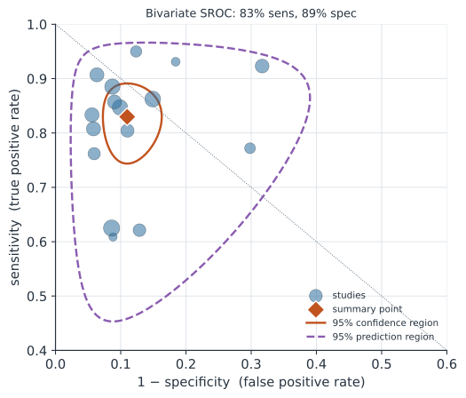
Different studies apply the test at different thresholds — a different cutoff on a continuous marker, a different reader, a different positivity rule. Raising the threshold catches fewer true positives (lower sensitivity) but also fewer false positives (higher specificity), so across studies sensitivity and specificity are negatively correlated: the points trace an ROC-shaped arc, not a cloud (Figure 1). Pooling sensitivity and specificity in two separate univariate meta-analyses ignores this correlation and mistakes threshold variation for disagreement, biasing both summaries toward the middle of the curve.

The bivariate model#

Model each study’s logit sensitivity and logit specificity as a draw from a bivariate normal (Reitsma et al. 2005):

$$\begin{pmatrix} \operatorname{logit}\text{se}_i \\ \operatorname{logit}\text{sp}_i \end{pmatrix} \sim \mathcal{N}\!\left( \begin{pmatrix} \mu_{\text{se}} \\ \mu_{\text{sp}} \end{pmatrix},\; \Sigma \right), \qquad \Sigma = \begin{pmatrix} \tau_{\text{se}}^2 & \rho\,\tau_{\text{se}}\tau_{\text{sp}} \\ \rho\,\tau_{\text{se}}\tau_{\text{sp}} & \tau_{\text{sp}}^2 \end{pmatrix},$$

with the observed counts drawn binomially from each study’s true sensitivity and specificity. The mean vector gives the summary operating point — pooled sensitivity $\operatorname{logit}^{-1}\mu_{\text{se}}$ and specificity $\operatorname{logit}^{-1}\mu_{\text{sp}}$ — while $\Sigma$ captures both the between-study heterogeneity ($\tau$) and the threshold correlation ($\rho < 0$). The logit scale handles the boundary (proportions near 0 or 1) and makes the normal approximation reasonable; the two-level structure is exactly a hierarchical model with a bivariate random effect. For a single, common threshold model the bivariate and HSROC parameterizations are algebraically equivalent — HSROC writes the same information as a summary ROC curve rather than a point.

Summary point, curve, and two regions#

The bivariate fit yields three things to report, and the distinction between the last two is often muddled:

• The summary operating point (pooled sensitivity, specificity).
• The 95% confidence region — uncertainty in the mean operating point, which shrinks with more studies.
• The 95% prediction region — where a new study’s operating point is expected to fall, reflecting genuine between-study heterogeneity; it stays wide even with many studies and is the honest picture of how much accuracy varies.

A worked example#

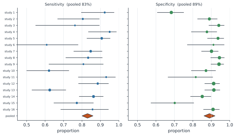
Sixteen studies of a test with a threshold effect, fit with the bivariate model.

import numpy as np
import jax.numpy as jnp
from jax import random
import numpyro
import numpyro.distributions as dist
from numpyro.infer import MCMC, NUTS

rng = np.random.default_rng(15)
k = 16
cov = np.array([[0.7**2, -0.5 * 0.7 * 0.6], [-0.5 * 0.7 * 0.6, 0.6**2]])
theta = rng.multivariate_normal([1.7, 2.0], cov, k)              # logit se, logit sp
sens, spec = 1 / (1 + np.exp(-theta[:, 0])), 1 / (1 + np.exp(-theta[:, 1]))
n_dis, n_hlth = rng.integers(20, 120, k), rng.integers(30, 200, k)
TP, FP = rng.binomial(n_dis, sens), rng.binomial(n_hlth, 1 - spec)

def bivariate(TP, nd, FP, nh):
    mu = numpyro.sample("mu", dist.Normal(jnp.array([1.5, 1.5]), 2.0).to_event(1))
    tau = numpyro.sample("tau", dist.HalfNormal(jnp.array([1.0, 1.0])).to_event(1))
    L = numpyro.sample("L", dist.LKJCholesky(2, concentration=2.0))
    with numpyro.plate("studies", len(TP)):
        th = numpyro.sample("th", dist.MultivariateNormal(mu, scale_tril=tau[..., None] * L))
        numpyro.sample("tp", dist.Binomial(nd, 1 / (1 + jnp.exp(-th[:, 0]))), obs=TP)
        numpyro.sample("fp", dist.Binomial(nh, 1 / (1 + jnp.exp(th[:, 1]))), obs=FP)

mcmc = MCMC(NUTS(bivariate), num_warmup=1000, num_samples=2000, num_chains=1,
            progress_bar=False)
mcmc.run(random.PRNGKey(0), jnp.array(TP), jnp.array(n_dis), jnp.array(FP), jnp.array(n_hlth))
s = mcmc.get_samples()
mu, L = np.array(s["mu"]), np.array(s["L"])
expit = lambda x: 1 / (1 + np.exp(-x))
corr = L[:, 1, 0] / np.sqrt(L[:, 1, 0]**2 + L[:, 1, 1]**2)
print(f"pooled sensitivity {expit(mu[:, 0]).mean()*100:.1f}% "
      f"[{np.percentile(expit(mu[:, 0]), 2.5)*100:.0f}, {np.percentile(expit(mu[:, 0]), 97.5)*100:.0f}]")
print(f"pooled specificity {expit(mu[:, 1]).mean()*100:.1f}% "
      f"[{np.percentile(expit(mu[:, 1]), 2.5)*100:.0f}, {np.percentile(expit(mu[:, 1]), 97.5)*100:.0f}]")
print(f"between-study threshold correlation {corr.mean():.2f}")

pooled sensitivity 82.8% [76, 88]
pooled specificity 88.9% [85, 92]
between-study threshold correlation -0.16

The model returns a summary sensitivity and specificity with credible intervals and a negative threshold correlation — and, crucially, the machinery to draw the prediction region that a pair of separate meta-analyses cannot (Figure 2).

In code#

R#

library(mada)                          # reitsma() fits the bivariate model
fit <- reitsma(data)                   # data: TP, FP, FN, TN per study
summary(fit)                           # summary sensitivity/specificity, correlation
plot(fit, sroccex = TRUE)              # the SROC curve with confidence & prediction regions
# metafor::rma.mv and lme4::glmer (a bivariate GLMM) fit the same model

Julia#

using Turing, LinearAlgebra
# a hierarchical bivariate-normal model on (logit sens, logit spec) with
# binomial observations — the same structure as the NumPyro model above

Why it matters#

Diagnostic accuracy reviews sit under real decisions: whether a rapid antigen test is good enough for community screening, whether a new assay can replace a reference standard, where to set a triage threshold. Getting the synthesis wrong — pooling sensitivity and specificity separately, or reporting a confidence region as if it were a prediction region — makes a test look more accurate and more consistent than it is, exactly the errors that push a mediocre test into practice. The bivariate/HSROC model is the standard (Cochrane’s method for diagnostic reviews) because it respects what a diagnostic study actually is: a single operating point on an ROC curve, measured with error, drawn from a heterogeneous population of thresholds.

Related#

• Meta-Analysis
• Diagnostic Testing and Screening
• Species Distribution Models: Presence–Absence Data
• Hierarchical Models
• Bayesian Inference
• ELISA
• Quantitative Methods