Discrete-Time Models and the Logistic Map

Many organisms breed in discrete seasons, and many diseases are tracked generation by generation, so their dynamics are naturally written as a rule mapping this year’s state to next year’s. These maps are simple to iterate yet capable of astonishingly rich behavior — including deterministic chaos from a one-line equation.

Geometric growth#

The discrete analogue of exponential growth is geometric growth, $$N_{t+1}=\lambda N_t,$$ which generates the sequence $N_t=\lambda^t N_0$. Here $\lambda$ is the finite (per-generation) growth rate; it links to the continuous intrinsic rate by $\lambda=e^{r}$. The population grows when $\lambda>1$, shrinks when $\lambda<1$, and holds steady when $\lambda=1$.

The Ricker model#

Real populations are density-dependent, and the Ricker model builds crowding into a discrete map, $$N_{t+1}=N_t\,e^{r(1-N_t/K)}.$$ When $N_t$ is small the exponent is near $r$ and growth is nearly geometric; as $N_t$ approaches the carrying capacity $K$ the exponent goes to zero and $N_{t+1}\approx N_t$. Unlike the smooth continuous logistic, overshoot in the Ricker map can produce oscillations and, for large $r$, chaos.

The logistic map#

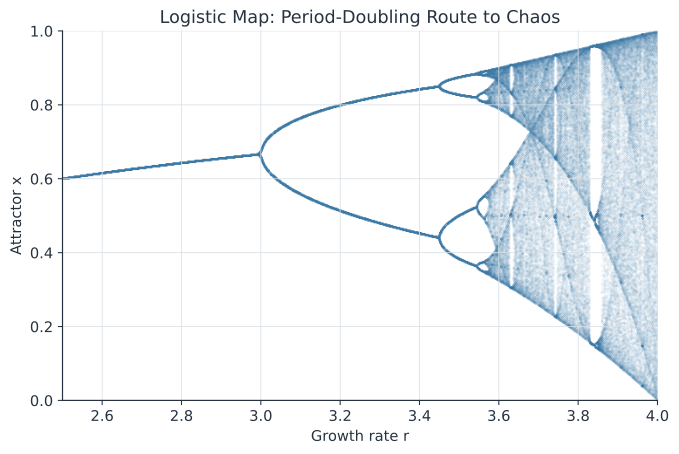
The most famous discrete model is the logistic map, $$x_{t+1}=r\,x_t(1-x_t),$$ where $x_t\in[0,1]$ is a scaled population fraction and $r$ is a growth parameter (here $0\le r\le 4$). Robert May’s 1976 analysis of this map showed that even a trivial nonlinear rule can produce cycles and chaos, reshaping how ecologists think about complexity and predictability.

Fixed points and stability#

A fixed point $x^*$ satisfies $x^*=f(x^*)$ with $f(x)=rx(1-x)$. Solving $x^*=rx^*(1-x^*)$ gives two fixed points: $x^*=0$ and $x^*=1-1/r$ (the latter positive only when $r>1$). Stability of a discrete map depends on the slope at the fixed point: $x^*$ is stable when $$|f'(x^*)|<1.$$ Here $f'(x)=r(1-2x)$. At $x^*=0$, $f'(0)=r$, so the origin is stable only for $r<1$. At $x^*=1-1/r$, $f'(x^*)=r\bigl(1-2(1-1/r)\bigr)=2-r$, so this nonzero fixed point is stable when $|2-r|<1$, i.e. for $1<r<3$.

Period-doubling and chaos#

As $r$ increases past $3$ the fixed point loses stability and a stable 2-cycle appears; past $\approx 3.449$ a 4-cycle; then 8, 16, and so on, with the thresholds bunching up in a period-doubling cascade. Beyond $r\approx 3.569$ the dynamics become chaotic — bounded, aperiodic, and sensitive to initial conditions. Each loss of stability is a bifurcation, and plotting the long-run attractor against $r$ produces the classic bifurcation diagram.

Cobweb plots#

A cobweb plot visualizes iteration: draw $y=f(x)$ and the line $y=x$, then bounce between them (up to the curve, across to the diagonal) to trace the orbit. Converging staircases spiral into a stable fixed point; diverging ones reveal cycles or chaos.

A worked example#

Take the logistic map with $r=2.5$. The nonzero fixed point is $x^*=1-1/r=1-1/2.5=1-0.4=0.6$. Its stability slope is $f'(x^*)=2-r=2-2.5=-0.5$, and since $|-0.5|<1$ the fixed point is stable — orbits converge to $0.6$. Now take $r=3.2$: the fixed point $x^*=1-1/3.2=0.6875$ has slope $2-3.2=-1.2$, and $|-1.2|>1$, so it is unstable; the map instead settles onto a stable 2-cycle.

In code#

We iterate the map and build the bifurcation diagram by plotting late iterates over a range of $r$.

R#

logmap <- function(x, r) r * x * (1 - x)

# converge to the fixed point 0.6 when r = 2.5
x <- 0.1
for (i in 1:100) x <- logmap(x, 2.5)
round(x, 6)   # 0.6

# bifurcation diagram
rs <- seq(2.8, 4.0, length.out = 600)
plot(NULL, xlim = range(rs), ylim = c(0, 1), xlab = "r", ylab = "x")
for (r in rs) {
  x <- 0.2
  for (i in 1:300) x <- logmap(x, r)          # transient
  for (i in 1:200) { x <- logmap(x, r); points(r, x, pch = ".") }
}

Python#

import numpy as np

def logmap(x, r):
    return r * x * (1 - x)

x = 0.1
for _ in range(100):
    x = logmap(x, 2.5)
print(round(x, 6))   # 0.6  -> stable fixed point

# bifurcation diagram data
rs = np.linspace(2.8, 4.0, 600)
R, X = [], []
for r in rs:
    x = 0.2
    for _ in range(300):        # discard transient
        x = logmap(x, r)
    for _ in range(200):
        x = logmap(x, r)
        R.append(r); X.append(x)
# plt.plot(R, X, ',k')  -> period-doubling route to chaos

0.6

Julia#

logmap(x, r) = r * x * (1 - x)

x = 0.1
for _ in 1:100
    x = logmap(x, 2.5)
end
round(x, digits = 6)   # 0.6

rs = range(2.8, 4.0; length = 600)
R = Float64[]; X = Float64[]
for r in rs
    x = 0.2
    for _ in 1:300; x = logmap(x, r); end       # transient
    for _ in 1:200
        x = logmap(x, r)
        push!(R, r); push!(X, x)
    end
end
# scatter(R, X; markersize = 0.5)  -> bifurcation diagram

Why it matters#

Discrete maps are the right tool for seasonally breeding populations and generation-based disease models, and they force us to check stability with the slope condition $|f'(x^*)|<1$ rather than the sign of a derivative. The logistic map is a canonical warning that simple, fully deterministic ecological rules can generate irregular, effectively unpredictable dynamics — a lesson that carries directly into forecasting outbreaks and managed populations.

Related#

• Exponential and Logistic Growth
• Equilibria and Stability
• Bifurcations
• Sequences
• Quantitative Methods