Spatial Synchrony and the Moran Effect

Asynchrony among patches stabilizes a metapopulation, because when one patch crashes another can rescue it. Spatial synchrony is the opposite and the danger: when populations across a region rise and fall in step, a bad year hits everywhere at once and the rescue effect vanishes, so regional extinction risk climbs. Synchrony can arise from a shared environment, from dispersal that couples neighboring populations, or from a common predator, and its epidemiological signature is the travelling wave of measles or influenza spreading out from large cities.

Left: two coupled oscillators whose phase difference drifts at weak coupling but locks to a constant once coupling exceeds the detuning. Center: between-patch synchrony rising with the correlation of environmental noise (the Moran effect), with dispersal adding a baseline. Right: a schematic travelling-wave phase map, with epidemic phase lagging with distance from a large source city.

What synchrony is and why it matters

Measure synchrony as the cross-correlation of the fluctuations of two populations around their own trends. A correlation near one means the patches move together; near zero means they move independently. Synchrony is the flip side of the inflationary effect of asynchrony: asynchronous patches let a metapopulation persist by averaging out local crashes, while synchronous patches remove that buffer, so simultaneous lows can drive the whole region extinct (Earn, Rohani & Grenfell 1998). The practical question is what makes distant populations synchronous in the first place.

The Moran effect

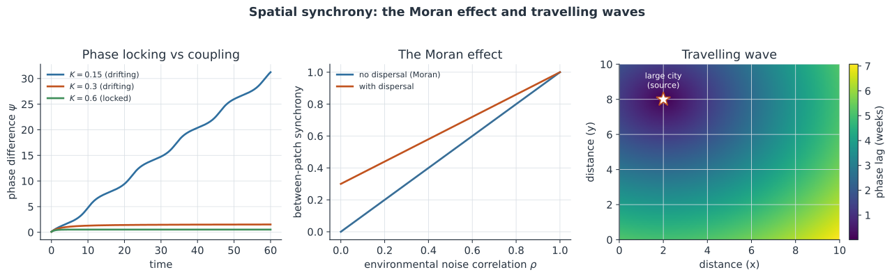
Take two populations with the same internal density-dependent structure, each driven by its own environmental noise, and let those noises be correlated (shared weather, say). Moran proved that if the density dependence is linear, the correlation of the two populations equals the correlation of the environmental noise driving them (Moran 1953). Synchrony is inherited from the environment with no dispersal at all: populations that never exchange a single individual still track each other because they experience correlated conditions. This is the Moran effect, and it is why species with similar dynamics synchronize over the spatial scale of the weather that forces them.

The assumptions matter: identical linear density dependence and additive noise. When density dependence is nonlinear, synchrony can be higher or lower than the noise correlation, but the qualitative lesson holds — correlated forcing buys synchrony for free.

Dispersal-induced synchrony and phase locking

Dispersal is the second route. Two population cycles behave like coupled oscillators: even weak coupling pulls their phases together, and once the coupling exceeds the mismatch in their natural frequencies, they phase-lock and oscillate in unison. Below that threshold the phase difference drifts around the cycle; above it, the phase difference settles to a constant. Dispersal and the Moran effect add up, so a little movement on top of a partly shared environment can lock populations that neither mechanism would synchronize alone.

Epidemic waves and spatial hierarchies

In epidemiology the same synchrony appears as travelling waves. Measles across pre-vaccination England and Wales rose and fell in a wave seeded from large cities, with the phase lag of a town growing with its distance from the urban core and shrinking with its own population size (Grenfell, Bjørnstad & Kappey 2001). Big cities are the pacemakers: they never fade out, so they force their smaller neighbors, and the epidemic ripples outward down the city-size hierarchy. Influenza shows the same structure, with spread tracking the flux of workers among population centers rather than simple geographic distance (Viboud et al. 2006).

A worked example

Simulate two identical Ricker patches, each forced by environmental noise, and vary only how correlated those two noise streams are. With a noise correlation of $\rho=0.2$ the patches fluctuate almost independently, and their population synchrony comes out near $0.19$ . Raise the noise correlation to $\rho=0.9$ and the population synchrony rises to about $0.86$ . The patches never exchange individuals, yet their abundances track the correlation of the shared environment — the Moran effect in one line of arithmetic.

In code

We drive two Ricker patches with environmental noise of a given correlation and measure the resulting cross-correlation of log abundances.

R

set.seed(1834)
r <- 1.8; K <- 100; sigma <- 0.25; steps <- 2000

synchrony <- function(rho) {
  L <- chol(matrix(c(1, rho, rho, 1), 2))   # correlate the two noise streams
  n <- c(50, 50); logs <- matrix(NA, steps, 2)
  for (t in seq_len(steps)) {
    eps <- as.numeric(t(L) %*% rnorm(2))
    n <- n * exp(r * (1 - n / K) + sigma * eps)
    logs[t, ] <- log(n)
  }
  x <- logs[-(1:200), ]
  cor(x[, 1], x[, 2])
}
sapply(c(0.2, 0.9), synchrony)   # synchrony tracks the noise correlation

Python

import numpy as np
import polars as pl

rng = np.random.default_rng(1834)
r, K, sigma, steps = 1.8, 100.0, 0.25, 2000


def synchrony(rho):
    # two Ricker patches driven by environmental noise of correlation rho
    L = np.linalg.cholesky([[1.0, rho], [rho, 1.0]])
    n = np.array([50.0, 50.0])
    logs = []
    for _ in range(steps):
        eps = L @ rng.standard_normal(2)
        n = n * np.exp(r * (1 - n / K) + sigma * eps)
        logs.append(np.log(n))
    x = np.array(logs)[200:]                 # drop transient
    return np.corrcoef(x[:, 0], x[:, 1])[0, 1]


rows = [{"noise_corr": rho, "pop_synchrony": round(synchrony(rho), 3)}
        for rho in (0.2, 0.9)]
print(pl.DataFrame(rows))

shape: (2, 2)
┌────────────┬───────────────┐
│ noise_corr ┆ pop_synchrony │
│ ---        ┆ ---           │
│ f64        ┆ f64           │
╞════════════╪═══════════════╡
│ 0.2        ┆ 0.189         │
│ 0.9        ┆ 0.859         │
└────────────┴───────────────┘

Julia

using LinearAlgebra, Random, Statistics

function synchrony(rho; r = 1.8, K = 100.0, sigma = 0.25, steps = 2000)
    rng = MersenneTwister(1834)
    L = cholesky([1.0 rho; rho 1.0]).L
    n = [50.0, 50.0]
    logs = zeros(steps, 2)
    for t in 1:steps
        eps = L * randn(rng, 2)
        n = n .* exp.(r .* (1 .- n ./ K) .+ sigma .* eps)
        logs[t, :] = log.(n)
    end
    x = logs[201:end, :]
    cor(x[:, 1], x[:, 2])
end

[synchrony(rho) for rho in (0.2, 0.9)]   # synchrony tracks noise correlation

Why it matters

Spatial synchrony sets the scale of risk. Synchronous populations share their fates, so conservation of a synchronized species cannot rely on rescue from elsewhere, and a synchronizing shock — a drought, a cold snap, a shared predator — can collapse a whole region at once. For pathogens the same synchrony is what makes measles and influenza epidemics predictable travelling waves keyed to city size and connectivity, and it is why breaking synchrony (staggering school terms, desynchronizing susceptible replenishment) can raise the chance that a pathogen fades out somewhere and fails to persist regionally.