Functional Responses and the Paradox of Enrichment

The Lotka–Volterra model assumes a predator eats prey in direct proportion to how many it meets, so its intake grows without bound. Real predators saturate: they need time to chase, subdue, and digest each meal, so their per-capita intake levels off as prey become abundant. That single change in the shape of the intake curve controls whether a consumer-resource system settles to a steady state or breaks into sustained cycles, and it produces the counterintuitive result that making a system more productive can make it less stable.

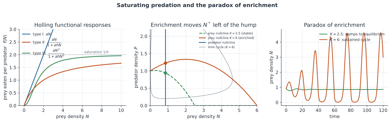
Left: the three Holling functional-response curves. Center: the Rosenzweig–MacArthur phase plane, where raising the prey carrying capacity slides the equilibrium left of the hump of the prey nullcline. Right: the prey time series switching from a damped approach to a sustained limit cycle as the carrying capacity increases.

The three functional responses

The functional response $f(N)$ is the number of prey a single predator eats per unit time as a function of prey density $N$ . Holling identified three shapes (Holling 1959).

Type I is linear, $f(N)=aN$ , with attack rate $a$ ; intake rises without limit. This is the mass-action term in the basic predator–prey model.
Type II saturates, $f(N)=\dfrac{aN}{1+ahN}$ , where $h$ is the handling time per prey; intake approaches the ceiling $1/h$ as prey become abundant.
Type III is sigmoid, $f(N)=\dfrac{aN^2}{1+ahN^2}$ ; predation is weak on rare prey (from switching to other food, learning, or prey refuges) and then saturates.

Deriving type II from the disc equation

Split a predator’s time budget between searching and handling. In a total time $T$ it captures $f$ prey, spending $hf$ of that time handling them, so only $T-hf$ is left to search. While searching, encounters accumulate at rate $aN$ per unit search time, giving $f=aN(T-hf)$ . Solving for the intake rate $f/T$ yields

$f(N)=\frac{aN}{1+ahN}.$

The attack rate $a$ sets the initial slope (how fast a predator finds prey), and the handling time $h$ sets the ceiling $1/h$ (how fast it can process them). A type I response is the $h\to 0$ limit, where handling is instantaneous and intake never saturates.

The Rosenzweig–MacArthur model

Give the prey logistic self-limitation and give the predator a type II response (Rosenzweig & MacArthur 1963).

$\begin{aligned} \frac{dN}{dt} &= rN\left(1-\frac{N}{K}\right) - \frac{aN}{1+ahN}\,P \\ \frac{dP}{dt} &= \frac{c\,aN}{1+ahN}\,P - mP \end{aligned}$

Here $r$ is the prey growth rate, $K$ the prey carrying capacity, $c$ the conversion efficiency, and $m$ the predator death rate. The interior equilibrium sits where the two nullclines cross. Setting $dP/dt=0$ with $P>0$ fixes the prey density on a vertical line,

$N^* = \frac{m}{a\,(c-mh)},$

which depends only on predator parameters, exactly as in the linear model. Setting $dN/dt=0$ gives the prey nullcline

$P = \frac{r}{a}\left(1-\frac{N}{K}\right)(1+ahN),$

a hump-shaped curve: it rises at low $N$ because saturation frees predators from each meal, then falls as prey approach $K$ . The peak of the hump lies at $N_{\text{hump}}=\dfrac{K}{2}-\dfrac{1}{2ah}$ , which moves right as $K$ grows.

The paradox of enrichment

Whether the equilibrium is stable turns on which side of the hump it sits on. If the vertical predator nullcline crosses the prey nullcline to the right of the peak, the equilibrium is stable and trajectories spiral in. If it crosses to the left of the peak, the equilibrium is unstable: the system undergoes a Hopf bifurcation and settles onto a stable limit cycle.

Because $N^*$ is fixed by predator parameters while $N_{\text{hump}}$ grows with $K$ , enriching the prey (raising $K$ ) eventually pushes the peak past $N^*$ and destabilizes the equilibrium — the paradox of enrichment (Rosenzweig 1971). Adding resources does not raise the steady prey level; it inflates the cycles until the troughs run so low that demographic noise can drive either species extinct. More food makes the system less persistent, not more.

A worked example

Take $r=1$ , $a=1$ , $h=0.5$ , $c=0.5$ , and $m=0.3$ in scaled units. The predator nullcline sits at

$N^* = \frac{m}{a(c-mh)} = \frac{0.3}{1\cdot(0.5-0.3\cdot 0.5)} = \frac{0.3}{0.35} \approx 0.857.$

The hump peaks at $N_{\text{hump}}=K/2-1/(2ah)=K/2-1$ . At $K=2.5$ the peak is at $0.25<N^*$ , so the equilibrium lies to the right of the hump and is stable. At $K=6$ the peak is at $2>N^*$ , so the equilibrium lies to the left and the system cycles. Enriching from $K=2.5$ to $K=6$ crosses the Hopf bifurcation.

In code

We integrate the model at both carrying capacities and test stability by the sign of the leading eigenvalue real part of the Jacobian at the interior equilibrium.

R

library(deSolve)
library(rootSolve)  # jacobian.full

rm_model <- function(t, y, p) {
  with(as.list(c(y, p)), {
    f <- a * N / (1 + a * h * N)
    list(c(r * N * (1 - N / K) - f * P, cc * f * P - m * P))
  })
}

p <- c(r = 1, a = 1, h = 0.5, cc = 0.5, m = 0.3)
Nstar <- p["m"] / (p["a"] * (p["cc"] - p["m"] * p["h"]))
for (K in c(2.5, 6)) {
  pk <- c(p, K = K)
  Pstar <- (p["r"] / p["a"]) * (1 - Nstar / K) * (1 + p["a"] * p["h"] * Nstar)
  J <- jacobian.full(y = c(N = Nstar, P = Pstar),
                     func = rm_model, parms = pk)
  cat(K, max(Re(eigen(J)$values)) < 0, "\n")  # TRUE = stable
$}

Python

import numpy as np
import polars as pl

r, a, h, c, m = 1.0, 1.0, 0.5, 0.5, 0.3
Nstar = m / (a * (c - m * h))          # predator nullcline


def jacobian(N, P, K):
    denom = 1 + a * h * N
    f = a * N / denom
    dfdN = a / denom**2                # d/dN of the type II response
    return np.array([
        [r * (1 - 2 * N / K) - dfdN * P, -f],
        [c * dfdN * P,                    c * f - m],
    ])


rows = []
for K in (2.5, 6.0):
    Pstar = (r / a) * (1 - Nstar / K) * (1 + a * h * Nstar)
    lead = np.linalg.eigvals(jacobian(Nstar, Pstar, K)).real.max()
    rows.append({"K": K, "lead_real": round(lead, 4),
                 "state": "stable" if lead < 0 else "limit cycle"})

print(pl.DataFrame(rows))

shape: (2, 3)
┌─────┬───────────┬─────────────┐
│ K   ┆ lead_real ┆ state       │
│ --- ┆ ---       ┆ ---         │
│ f64 ┆ f64       ┆ str         │
╞═════╪═══════════╪═════════════╡
│ 2.5 ┆ -0.0729   ┆ stable      │
│ 6.0 ┆ 0.0571    ┆ limit cycle │
└─────┴───────────┴─────────────┘

Julia

using DifferentialEquations, LinearAlgebra

r, a, h, c, m = 1.0, 1.0, 0.5, 0.5, 0.3
Nstar = m / (a * (c - m * h))

function jac(N, P, K)
    denom = 1 + a * h * N
    f = a * N / denom
    dfdN = a / denom^2
    [r * (1 - 2N / K) - dfdN * P   -f;
     c * dfdN * P                   c * f - m]
end

for K in (2.5, 6.0)
    Pstar = (r / a) * (1 - Nstar / K) * (1 + a * h * Nstar)
    lead = maximum(real, eigvals(jac(Nstar, Pstar, K)))
    println(K, "  ", lead < 0 ? "stable" : "limit cycle")
end

Why it matters

Saturating intake is the rule, not the exception, wherever a consumer must handle its resource: predators subduing prey, parasitoids attacking hosts, or transmission saturating when each infectious host can only contact so many others per day. The paradox of enrichment warns that raising productivity — fertilizing a lake, feeding a host population, boosting a reservoir — can trade a stable steady state for large-amplitude cycles that raise extinction and fade-out risk. Type III responses and prey refuges pull in the other direction, restoring low-density stability, which is why refugia and switching matter for both biological control and pathogen persistence.