Compartmental Models

Compartmental models have many shapes and sizes. They divide a population into distinct compartments — groups defined by their status with respect to a disease — and describe how individuals move between them over time. Despite their simplicity, compartmental models are one of the most powerful tools in infectious disease ecology and epidemiology.

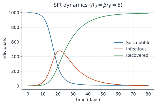
The SIR model#

The classic example is the SIR model, which divides a population into three compartments:

• S — Susceptible: individuals who can become infected
• I — Infectious: individuals who are infected and can transmit
• R — Recovered (or removed): individuals who are no longer susceptible or infectious

Individuals flow from $S \to I \to R$. The dynamics are governed by a system of ordinary differential equations:

$$\begin{aligned} \frac{dS}{dt} &= -\beta \frac{S I}{N} \\ \frac{dI}{dt} &= \beta \frac{S I}{N} - \gamma I \\ \frac{dR}{dt} &= \gamma I \end{aligned}$$

where $\beta$ is the transmission rate, $\gamma$ is the recovery rate, and $N = S + I + R$ is the total population size.

The basic reproduction number#

A key quantity derived from the model is the basic reproduction number, $R_0$ — the average number of secondary infections produced by a single infectious individual in a fully susceptible population. For the SIR model,

$$R_0 = \frac{\beta}{\gamma}$$

When $R_0 > 1$, an outbreak can grow; when $R_0 < 1$, it dies out.

Where does $\beta/\gamma$ come from? Two short arguments give it — one counting infections directly, one falling out of the threshold for growth.

Show the derivation

Rate times duration. Drop a single infectious individual into an otherwise fully susceptible population, so $S \approx N$ and the susceptible fraction $S/N \approx 1$. That individual transmits by mass action at rate $\beta \, S/N \approx \beta$ — that many new infections per unit time. Recovery is a constant-rate process ($\gamma I$ leaves the infectious class per unit time), so the time spent infectious is exponentially distributed with mean

$$\mathbb{E}[\text{infectious period}] = \frac{1}{\gamma}.$$

The expected number of secondary infections is the transmission rate multiplied by how long transmission lasts:

$$R_0 = \underbrace{\beta}_{\text{infections per unit time}} \times \underbrace{\frac{1}{\gamma}}_{\text{mean infectious period}} = \frac{\beta}{\gamma}.$$

The threshold for growth. The same number governs whether the outbreak takes off, which is why $R_0 = 1$ is the dividing line. Early on $S \approx N$, so the infectious equation

$$\frac{dI}{dt} = \beta \frac{S}{N} I - \gamma I$$

linearizes to

$$\frac{dI}{dt} \approx (\beta - \gamma)\, I ,$$

an exponential with growth rate $\beta - \gamma$. Infections grow when $\beta - \gamma > 0$, i.e. when

$$\frac{\beta}{\gamma} > 1 .$$

Defining $R_0 = \beta/\gamma$ makes “the epidemic grows” and “$R_0 > 1$” the same statement.

Both routes assume $S \approx N$: $R_0$ is defined in a fully susceptible population. Once susceptibles deplete, the relevant quantity is the effective reproduction number $R_t = R_0 \, S/N$, and the epidemic peaks exactly when $S/N$ falls to $1/R_0$ so that $R_t = 1$. For models with more than one infected compartment, this “rate times duration” bookkeeping is done with a matrix — see The Next-Generation Matrix and R₀.

Extensions#

The SIR framework extends naturally to capture more biological detail:

• SEIR — adds an Exposed (latent) compartment for diseases with an incubation period
• SIS — allows individuals to return to the susceptible class (no lasting immunity)
• SIRS — adds waning immunity, returning recovered individuals to susceptible
• Vital dynamics — births and deaths for longer time horizons
• Vector, spatial, and stochastic variants for more realistic systems

Analyzing model behavior#

To understand a model’s long-term behavior, we identify its equilibria and study their stability. This is done by linearizing the system and examining the Jacobian matrix, which shows how the SIR model can be analyzed at the disease-free equilibrium.

Related#

• Jacobians — stability analysis for the SIR model
• The Next-Generation Matrix and R₀
• Equilibria and Linear Stability
• Exponential and Logistic Growth
• Bifurcations — the $R_0=1$ threshold
• SEIR and Compartmental Extensions
• Within-Host Dynamics and the Immune Response
• Vector-Borne Disease Models
• Stochastic Epidemics and the Gillespie Algorithm
• The Effective Reproduction Number and Forecasting
• Fitting Dynamic Models to Data
• Pharmacokinetics: Compartment Models — the same compartment framework applied to drugs
• Mathematical Biology (BIO 301) — the course where these models are developed in depth