G-Estimation
G-estimation is the third of Robins’ g-methods — alongside the g-formula (standardization) and inverse-probability weighting of marginal structural models — and the one that feels least like ordinary regression. It estimates the parameters of a structural nested model by asking a clean counterfactual question: what value of the treatment effect would make treatment look unrelated to the outcome it would have had under no treatment? Like IPW, it is built for time-varying confounding; unlike IPW, it handles effect modification gracefully and is often more efficient.
The treatment-free outcome#
A structural nested mean model parameterizes the effect of treatment as a blip: how much treatment shifts the mean outcome relative to never being treated. In the simplest one-parameter form, the effect of a binary is per unit, and the treatment-free (counterfactual) outcome is
the outcome you would have seen under no treatment — if is the true effect. Under no unmeasured confounding, that counterfactual outcome is independent of the treatment actually received, conditional on the confounders : treatment was assigned based on , not on the untreated potential outcome.
The estimating equation#
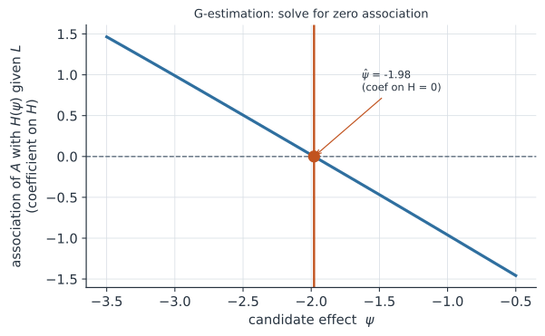
G-estimation turns that independence into an equation to solve. For a candidate , compute and test whether it still predicts treatment given — for instance, via the coefficient on in a logistic regression of on and . The g-estimate is the value that drives that coefficient to zero (Figure 1):
Because the criterion is a single monotone function of , a grid search or a bisection finds it immediately, and inverting the test gives a confidence interval. The logic relies on rank preservation in its simplest form, but the mean-model version needs only the conditional-independence assumption above.
One of three g-methods#
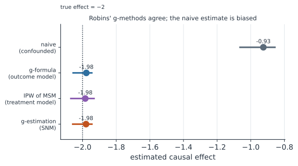
On the running confounded example (true effect ), g-estimation, the g-formula, and IPW all recover the truth while the naive comparison is badly biased (Figure 2). They differ in what they model:
- g-formula models the outcome (standardize predicted outcomes over the confounder distribution);
- IPW models the treatment (reweight by the inverse propensity);
- g-estimation also models the treatment, but through the structural nested model, which makes doubly-robust and effect-modification extensions natural.
A worked example#
import numpy as np
import statsmodels.api as sm

rng = np.random.default_rng(2)
n = 4000
L = rng.normal(0, 1, n)
A = rng.binomial(1, 1 / (1 + np.exp(-0.8 * L)))
Y = -2.0 * A + 1.5 * L + rng.normal(0, 1, n)     # true effect = -2

# g-estimation: find psi such that H(psi) = Y - psi*A is unrelated to A given L
def coef_on_H(psi):
    H = Y - psi * A
    return sm.Logit(A, sm.add_constant(np.c_[L, H])).fit(disp=0).params[-1]

lo, hi = -4.0, 0.0                                # bisection for the zero crossing
for _ in range(40):
    mid = (lo + hi) / 2
    if coef_on_H(mid) > 0:
        lo = mid
    else:
        hi = mid
print(f"g-estimate psi = {(lo + hi) / 2:+.2f}   (true -2.00)")
g-estimate psi = -1.98 (true -2.00)
The estimating equation lands on : the effect that, once subtracted off, leaves treatment and the treatment-free outcome unrelated given .
In code#
R#
# gesttools / DTRreg implement g-estimation of structural nested models,
# including the time-varying, multi-stage case
library(DTRreg)
fit <- DTRreg(Y, blip.mod = list(~1), treat.mod = list(A ~ L),
              tf.mod = list(~L), data = d, method = "gest")
summary(fit)     # the blip (effect) parameter psi
Julia#
using GLM, DataFrames
coef_on_H(psi) = coef(glm(@formula(A ~ L + H), transform(d, :Y => (y -> y .- psi .* d.A) => :H),
                         Binomial()))[end]
# bisect coef_on_H over psi to its zero crossing
Why it matters#
When treatment and a time-varying confounder chase each other over time — CD4 count driving HIV therapy while therapy raises CD4, disease severity driving a drug while the drug changes severity — the ordinary instinct to “adjust for the confounder” fails, and the g-methods are the correct tools. G-estimation is the member of that family that most directly targets the causal effect rather than a weighted average, extends cleanly to effect modification (does the effect differ by subgroup?), and underlies the analysis of dynamic treatment regimes — rules that say treat when the biomarker crosses a threshold. It is more demanding to implement than IPW, which is why it is less common, but on exactly the problems these methods exist for, it is often the more efficient and flexible choice.