Inverse Probability Weighting
Inverse probability weighting (IPW) removes confounding by reweighting. Each unit is weighted by the inverse of the probability of the treatment it actually received, which up-weights the under-represented combinations of treatment and confounders and down-weights the over-represented ones — building a pseudo-population in which treatment is no longer associated with the measured confounders. It is the same idea as reweighting a biased survey to represent the target population, applied to a treatment instead of a sampling design, and it reuses the propensity score as its engine.
The pseudo-population and the weights#
With propensity , assign each unit the inverse-probability weight
In the weighted sample, treatment and confounders are independent, so a simple weighted difference in outcomes estimates the causal effect:
the Hájek (self-normalized) estimator, generally preferred to the plain Horvitz–Thompson version because it is less sensitive to a few large weights. The same assumptions as any propensity method apply — no unmeasured confounding and positivity — and positivity bites harder here, because a propensity near or produces a colossal weight.
Stabilized weights#
Raw weights can be wildly variable, and a handful of huge ones wreck the variance. Stabilized weights replace the numerator with the marginal probability of the treatment received,
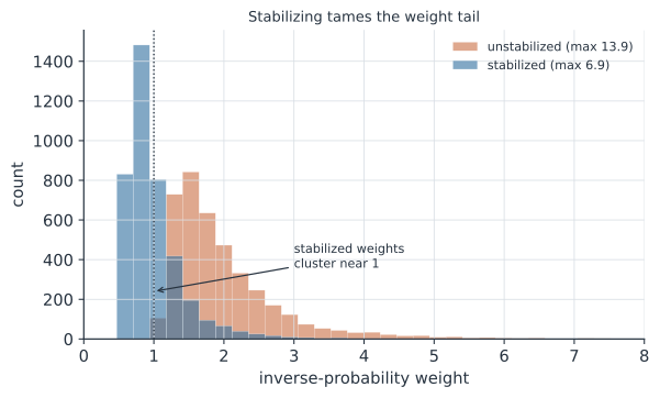
which leaves the balancing property intact but pulls the weights toward , sharply cutting variance (Figure 1). When extreme weights remain, truncate them at, say, the 1st and 99th percentiles — trading a little bias for a lot of stability.
Marginal structural models#
Weighting generalizes past a single binary contrast. Fit an outcome model — a marginal structural model (MSM) — in the weighted pseudo-population, e.g. , and its coefficients are marginal (population-level) causal effects, not the conditional-on- effects a plain outcome regression would give. The MSM can carry continuous exposures, interactions, and — crucially — treatment histories.
Time-varying treatments: the reason IPW exists#
The setting IPW was really built for is a treatment given repeatedly over time, with a time-varying confounder that is itself affected by earlier treatment (Robins, Hernán & Brumback 2000). The canonical example: HIV treatment decided by CD4 count , while treatment also changes future CD4 (Figure 2).
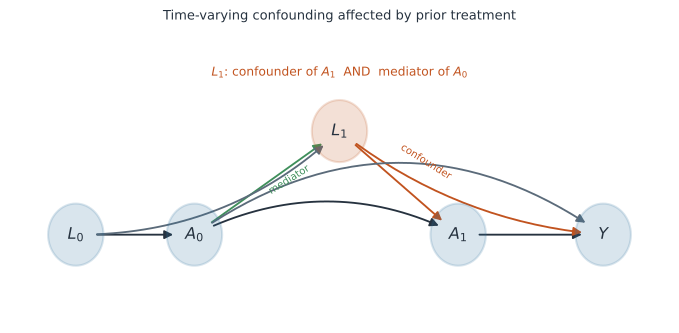
Here standard regression is stuck: you must adjust for to de-confound , but adjusting for blocks the effect of that runs through and conditions on a collider — biasing the estimate either way. Weighting sidesteps the trap: weight by the inverse probability of the whole treatment history and fit an MSM, and the time-varying confounders never enter the outcome model at all. G-estimation is the other principled solution to the same problem.
A worked example#
The point-treatment version, on the running confounded example (true effect ).
import numpy as np
import statsmodels.api as sm

rng = np.random.default_rng(2)
n = 4000
L = rng.normal(0, 1, n)
A = rng.binomial(1, 1 / (1 + np.exp(-0.8 * L)))
Y = -2.0 * A + 1.5 * L + rng.normal(0, 1, n)     # true ATE = -2

ehat = sm.Logit(A, sm.add_constant(L)).fit(disp=0).predict()
w = A / ehat + (1 - A) / (1 - ehat)              # inverse-probability weights
pA = A.mean()
sw = A * pA / ehat + (1 - A) * (1 - pA) / (1 - ehat)   # stabilized

def hajek(weight):
    return (np.sum(weight * A * Y) / np.sum(weight * A)
            - np.sum(weight * (1 - A) * Y) / np.sum(weight * (1 - A)))

print(f"naive              {Y[A==1].mean() - Y[A==0].mean():+.2f}")
print(f"IPW (unstabilized) {hajek(w):+.2f}   max weight {w.max():.1f}")
print(f"IPW (stabilized)   {hajek(sw):+.2f}   max weight {sw.max():.1f}   (true -2.00)")
naive              -0.93
IPW (unstabilized) -1.98   max weight 13.9
IPW (stabilized)   -1.98   max weight 6.9   (true -2.00)
Both weightings recover the true ; stabilizing barely moves the point estimate but shrinks the largest weight, which in a bigger or more extreme problem is the difference between a usable estimate and a hopelessly noisy one.
In code#
R#
library(WeightIt)         # weights + balance diagnostics; survey/ipw also common
W <- weightit(A ~ L, data = d, method = "glm", estimand = "ATE", stabilize = TRUE)
library(survey)
des <- svydesign(~1, weights = W$weights, data = d)
svyglm(Y ~ A, design = des)     # the marginal structural model
Julia#
using GLM, DataFrames
e = predict(glm(@formula(A ~ L), d, Binomial()))
d.w = @. d.A / e + (1 - d.A) / (1 - e)          # inverse-probability weights
lm(@formula(Y ~ A), d, wts = d.w)               # weighted outcome model (the MSM)
Why it matters#
Inverse probability weighting is the standard tool for causal questions with treatment sustained over time — antiretroviral therapy, statins, occupational exposures — where the thing that decides today’s treatment is itself moved by yesterday’s, and ordinary regression cannot give an unbiased answer. Even for a single time point it has a clean interpretation (a reweighted pseudo-experiment) and pairs naturally with an outcome model to become doubly robust. Its Achilles heel is positivity: when some units almost never receive a given treatment, their inverse weights explode, and no amount of stabilizing rescues an estimate that is really being carried by three people.